
NGC 7293, The Helix Nebula ~4.5 hours of LHaRGB: Dealing with “Bad Data”
Date: January 10, 2022
Cosgrove’s Cosmos Catalog ➤#0094

This image achieved Explore Status on Flickr!
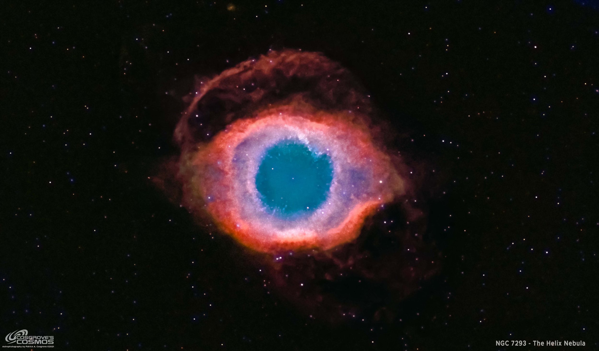
NGC 7293 - The Helix Nebula in LHaRGB. This image was a struggle using data that has all kinds of problems! (click to see high res version via Astrobin.com)
Table of Contents Show (Click on lines to navigate)
About the Target
NGC 7293, The Helix Nebula, is also known as Caldwell 63, “The Eye of God”, or the “Eye Of Sauron”. It is a planetary nebula located in the constellation of Aquarius. The distance from Earth to the Helix Nebula was determined to be ~655 light-years by the Gaia Mission.
Wikipedia provides an interesting overview of this object:
The Helix Nebula is an example of a planetary nebula, formed by an intermediate to low-mass star, which sheds its outer layers near the end of its evolution. Gases from the star in the surrounding space appear, from our vantage point, as if we are looking down a helix structure. The remnant central stellar core, known as the central star (CS) of the planetary nebula, is destined to become a white dwarf star. The observed glow of the central star is so energetic that it causes the previously expelled gases to brightly fluoresce.
The nebula is in the constellation of Aquarius, and lies about 650 light-years away, spanning about 0.8 parsecs (2.5 light-years). Its age is estimated to be 10600+2300
−1200 years, based on its measured expansion rate of 31 km·s−1.[6]
It continues:
The Helix Nebula is thought to be shaped like a prolate spheroid with strong density concentrations toward the filled disk along the equatorial plane, whose major axis is inclined about 21° to 37° from our vantage point. The size of the inner disk is 8×19 arcmin in diameter (0.52 pc); the outer torus is 12×22 arcmin in diameter (0.77 pc); and the outer-most ring is about 25 arcmin in diameter (1.76 pc). The outer-most ring appears flattened on one side due to it colliding with the ambient interstellar medium.[11]
Expansion of the whole planetary nebula structure is estimated to have occurred in the last 6,560 years, and 12,100 years for the inner disk.[12] Spectroscopically, the outer ring's expansion rate is 40 km/s, and about 32 km/s for the inner disk.
Knots
A closer view of knots in the nebula
The location of NGC 7293 (labelled in red)
The Helix Nebula was the first planetary nebula discovered to contain cometary knots.[13] Its main ring contains knots of nebulosity, which have now been detected in several nearby planetary nebulae, especially those with a molecular envelope like the Ring nebula and the Dumbbell Nebula.[14] These knots are radially symmetric (from the CS) and are described as "cometary", each centered on a core of neutral molecular gas and containing bright local photoionization fronts or cusps towards the central star and tails away from it.[15] All tails extend away from the Planetary Nebula Nucleus (PNN) in a radial direction. Excluding the tails, each knot is approximately the size of our Solar system, while each of the cusp knots are optically thick due to Lyc photons from the CS.[3][6][16] There are about 40,000 cometary knots in the Helix Nebula.[17]
The knots are probably the result of Rayleigh-Taylor instability. The low density, high expansion velocity ionized inner nebula is accelerating the denser, slowly expanding, largely neutral material which had been shed earlier when the star was on the Asymptotic Giant Branch.[18]
The excitation temperature varies across the Helix nebula.[19] The rotational-vibrational temperature ranges from 1800 K in a cometary knot located in the inner region of the nebula are about 2.5'(arcmin) from the CS, and is calculated at about 900 K in the outer region at the distance of 5.6'.[19]
The Annotated Image

This annotated image was created using the ImageSolver and AnnotateImage scripts in Pixinsight.
The Location in the Sky

This finding chart was created with the new FindingChart process in Pixinsight. The image rectangle is shown in red.
About the Project
Sometimes a project just does not seem to come together as you might have envisioned.
You have a plan. You set up. You capture your subs and cal frames. And despite your best efforts, the data set is just not as good as you hoped it would be.
This is one of those cases! I was pretty disappointed with this project.
Great images don’t come from poor data. But there is much you can do to get some kind of usable image out of data that is less than ideal - and that is the story of this image.
Since this image was a bit of a disappointment to me, I am not really thrilled to add it to the portfolio - but I made a commitment to myself to share both the good and the bad since everybody runs into this at some point - even extremely accomplished astrophotographers. I just show my work as it is - others may elect not to do this.
Why this Target?
I’ve always liked this object. The “Eye of God”, “The Eye of Sauron” - this image has a lot of drama to it!
Unfortunately, this is a very tough target for me to shoot because of my location and the characteristics of my driveway location:
It is low in the sky - at best, its higher elevation is only 26 degrees - so I am looking “edgewise” through a lot of atmosphere.
It is positioned right over my neighbor’s house across the street - and I get heat waves from his roof!
It is tightly framed between sets of trees lining my driveway - I can only get about 90 minutes of subs collected each night.
But I did shoot this target last year and I got a pretty pleasing image from it. It turned out to be a surprisingly popular image as well. You can see that project HERE. And here is the image I took then:
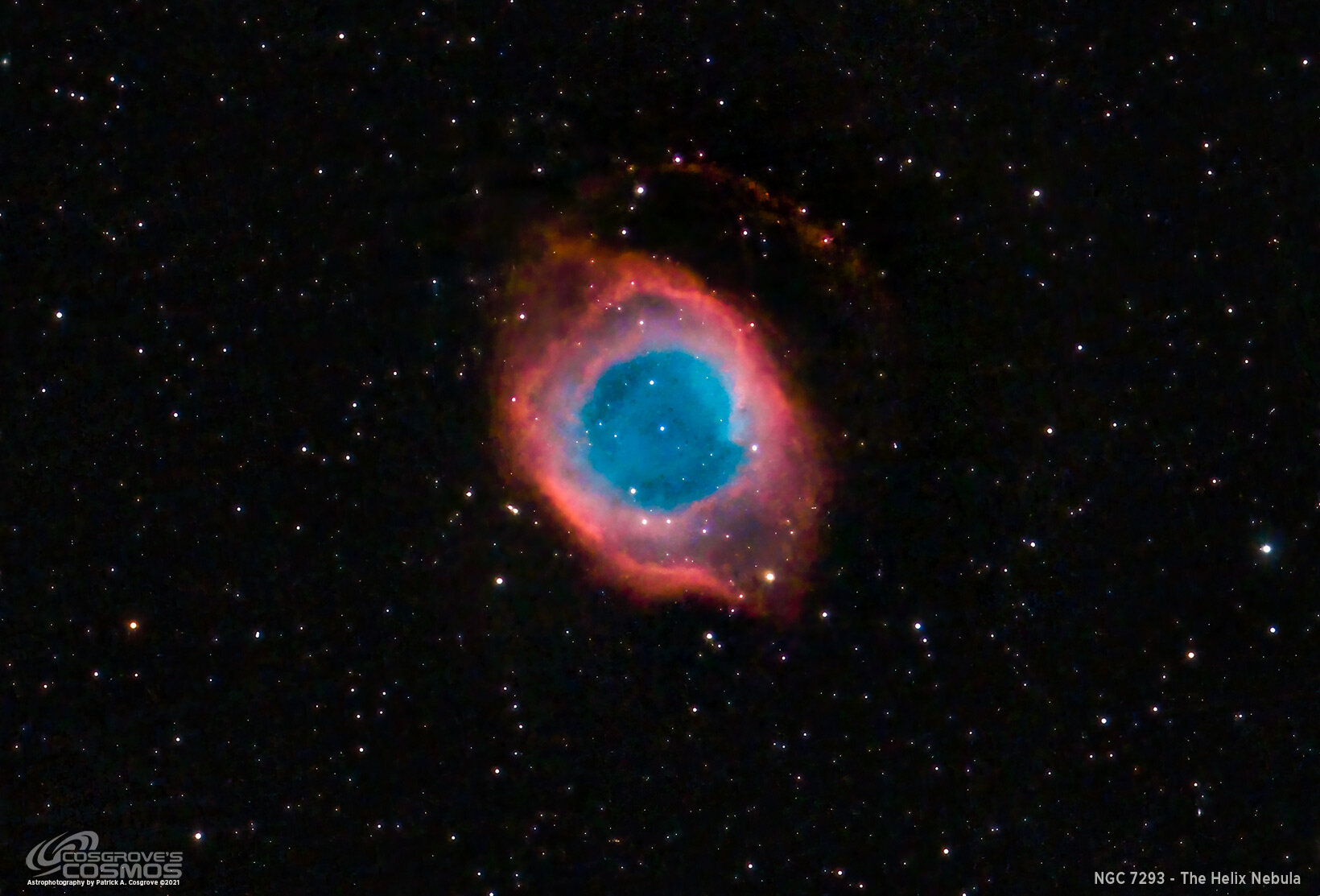
My first attempt on the Helix Nebula from October of 2020. Just short of two hours with a OSC camera.
The Current image for comparison.
I wanted to try this target again and see if I could improve on it. How was I planning on improving upon it?
Use a scope with a longer focal length (the Astro-Physics 130mm)
Do a longer integration
Use a next-generation mono camera - the ASI2600MM-Pro
Collect LRGB & Ha data
This should surely get me a substantial improvement over this first image - Right?
Data Collection
November is typically a miserable month for astrophotography here in Western New York.
But not this past November!
We had almost four clear moonless nights in a row - starting on November 5 and going through November 8th! The last night things began to deteriorate around 3 am, but since captures started around 7 pm that provided a full with hours of useful access to the sky. Simply amazing!
This is the ninth image I have processed from that what was captured at that time.
However, I knew at the time that the collection was NOT going well!
At that low altitude looking south, I was not only looking through a lot more atmosphere, I was also looking into a swirling mist of thin clouds. Even looking at the early subs I could see a lot of moving gradients and frames where all detail was wiped out! I was running into more issues than I had hoped.
Added to this, tree and branch growth over the last year had caused the tree lines to grow closer together and thus my time for target accessibility was reduced from before. This really messed up my collection plan - I ended up hitting the trees before I planned on and ended up being short on subs for certain filters.
I hoped our stretch of great weather would extend a few more days so I could grab some of the subs I had missed, but this was not to be. Knowing that the data was not as good as hoped, I kept putting off processing this data set in favor of others that were higher in the sky and had no such problems.
The Closer I look, the more problems I see!
As I dug into the data further - I found more issues. Apparently, during one night, I messed up my SGP setup and did not tell the software to do rotations when “centering” the scope. This meant that one night’s data was rotated differently than the other three nights. Sigh. More things to deal with.
I blinked all of the data and ended up throwing out a bunch of frames since thin clouds had wiped out all detail. On top of that, I found a weird noise pattern in the low code values of the Green Master image. I kept going back into ImageIntegration and changing the low rejection threshold to clean that up. I was able finally to do that.
But at end of the day, I had L, R, G, B, Ha data, but in some cases, I had way too few samples to make this work well. For example, I ended up with only 17 frames for the green filter!
The rotation problem with some of the frames would also cause me to really crop in pretty far - so if I had artifacts or noise issues, they would be very hard to miss!
Image Processing
I have found that if you are too aggressive with the image processing, the image suffers from it. It no longer looks natural or ethereal. Well, this image required a lot of heavy-handed image processing to minimize the data issues. Heavy-handed? I beat this puppy with a sledgehammer!
Extensive denoising was done at several phases of the processing.
The stars ended up looking funky - with color rings, and so I needed to address that.
Colors seemed very muted and to bring them out I had to play a lot of games.
Delicate wisps of nebulosity were muted and unsharp-looking.
Normally I keep a very orderly processing log - this makes it easy for me to share with you the processing I did. The processing here was NOT orderly at all. I tried A, I tried B, then I tried C. Then I went back to A and added a little C. And so on. In the end - I no longer had a clear processing path I could easily reconstruct. It was just … ugly.
In the processing section below, I did try and share what I did do, but I apologize that some of this was lost in the thrashing
Image Critique
Hmm. Where do I start….
I think this image is just an unfortunate lost opportunity.
My image processing did act to de-emphasize the worst problems with this image data set - but the colors are not “transparent”, the stars are still not where they need to be.
I would say that the new image is marginally better than my first attempt - but it is not at all what I had hoped for.
Frankly, I was pretty down on this image - maybe more so than I should be. I had shared this with a couple of my local astrophotography buddies and they thought I was being too hard on the image. Perhaps I am, but I know what I had hoped to achieve and these results have fallen far short of my hopes.
Note: the Image processing details section can be found at the end of this post.
Capture Details
Software
Capture Software: PHD2 Guider, Sequence Generator Pro controller
Image Processing: Pixinsight, Photoshop - assisted by Coffee, extensive processing indecision and second-guessing, editor regret and much swearing…..
Lights Frames
Taken the nights of November 5th-8th, 2021
55 x 90 seconds, bin 1x1 @ -15C, Gain 100.0, ZWO Gen II Lum Filter
45 x 90 seconds, bin 1x1 @ -15C, Gain 100.0, ZWO Gen II Red Filter
17 x 90 seconds, bin 1x1 @ -15C, Gain 100.0, ZWO Gen II Green Filter
22 x 90 seconds, bin 1x1 @ -15C, Gain 100.0, ZWO Gen II Blue Filter
13 x 300 seconds, bin 1x1 @ -15C, Gain 100.0, Astrodon 5nm Ha Filter
Total of 4 hours 38 minutes
Cal Frames
25 Darks at 300, bin 1x1, -15C, gain 100
25 Darks at 90 sec, bin 1x1, -15C, gain 100
25Dark Flats at Flat exposure times, bin 1x1, -15C, gain 100
Flats darks, 12 at each flat exposure time.
Capture Hardware
Click below to visit the Telescope Platform Version used for this image.
Scope: Astrophysics 130mm Starfire F/8.35 APO refractor
Guide Scope: Televue 76mm Doublet
Camera: ZWO AS2600mm-pro with ZWO 7x36 Filter wheel with ZWO LRGB filter set, Astrodon 5nm Ha & OIII, and Astronomiks 6nm SII Narrowband filter set
Guide Camera: ZWO ASI290Mini
Focus Motor: Pegasus Astro Focus Cube 2
Camera Rotator: Pegasus Astro Falcon
Mount: Ioptron CEM60
Polar Alignment: Polemaster camera
Image Processing Log
1. Blink Screening Process
All light images were reviewed with the Blink process.
Lum Subs
7 subs have thin cloud cover and significant detail loss - rejected
Some satellite trails but no problem expected
Cloud Gradients seen!
Red Subs:
3 removed for lack of detail
Gradients seen
Green Subs:
Not many frames! only 8
Frames there seem to look OK
Blue Subs:
Relatively few frames
Frames that are there look OK
Ha Subs
Everything looks pretty good
FLats, and Flat Darks, and Darks looked very good
2. WBPP 2.3 Run
all frames loaded
setup for calibration only - no integration
Cosmetic Correction setup
Pedastal image of 50 used for Ha images
Subframe weighting: psf signal - this is a new feature of version 2.3
Run complete with no issues

WBPP Calibration Panel

WBPP Lights Panel

WBPP Post-Process Panel
3. Image Integration
Because of Gradients seen, I am going to have to use NormailzedScaleGradient script for the Lum and Red Subs
I will use the normal ImageIntegration process for all other images.
Panels for each integration can be seen below.
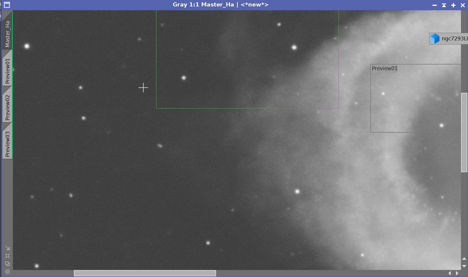
Note that the Green Master showed a strange linear noise pattern in some regions, so Image integrations were re-run several times to remove these artifacts.
Rotation problem seen in Blue and Lum data.

NormalizedScaleGradient set up for run on Lum Images

ImageIntegration Panel for Lum Image

Here is a sample of a gradient seen across one sample of the Lum images. The NormalizedScaleGradient will flatten these gradients out which means that ImagIntegration will be more successful in applying its rejection thresholding.

Lum Image Reject High map for Lum. Notice the satellite trail that was removed and the evidence that we have some frames with a different rotations that others.

NormalizedScaleGradient set up for the Red run

ImageIntegration set up for Red run,.

Here was the original set up for the ImageItegration Panel for the Green Subs. This was unsuccessful in removing some low end artifacts seen in the base signal of the image.

After some trial and error, I settled o a sigma low threshold of 2.0. This was successful in removing the artifacts seen.

Here is the Low rejection map for green after ImageIntegration had new sigma low parameters set.

The left image show a section of artifacts that can be seen in the low code values of the image. The image in the right has removed most evidence of these.

The Blue ImageIntegration Panel.

The Ha ImageItegration Panel.
4. Crop all of the images
Since we have rotation differences, we need to not only crop the image to get rid of ragged images, we need to crop deeply to eliminate unmatched image areas.
5. Dynamic Background Extraction
DBE was run for all images using Subtraction as the correction method.
The sampling plan was similar for each image but it was customized as needed. See an example sample plan below.
Lum image DBE sampling plan (click to enlarge)
Green Image DBE Sampling Plan (click to enlarge)
Ha Image DBE Sampling Plan (click to enlarge)
5. Deconvolution Prep for the L image.
I decided to use the L, R, G, & B images for the color image. Since the Ha layer had the most detail, I decided to use it for the L image I will fold in later when in the Nonlinear domain.
Object mask created
A nonlinear version of the image was created using STF->HT method
Use HT to clip blacks and push stars and nebula to white
Create Local protection images
Run StarMasks with layers = 6, all else default
Adjust star mask with HT to boost star size - move the middle arrow to the 25% point
Create PSF image with PSFImage Script.
Object Mask for Ha (click to enlarge)
Local support image for Ha (click to enlarge)
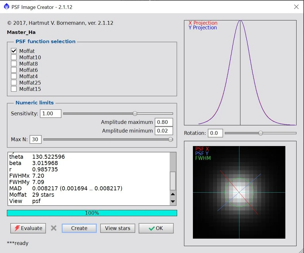
The PSFImage Panel creating the PSF image for Ha.

The final PSF image for Ha
6. Apply Deconvolution for the L image
For the Ha image
Apply Object mask to the image
Set psf to the right one for the image
add the right local support image
Create 3 preview sections on the image
Test different global dark settings until optimal found
0.025
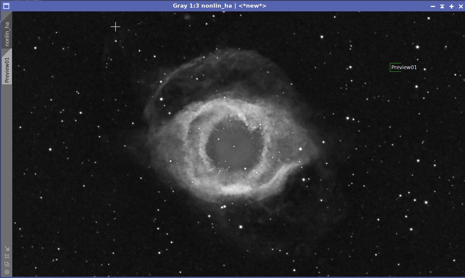
Ha image before Deconvolution
Ha image after deconvolution.
7. Run Denoise on the L image
Run EZ-Denoise on the Ha Image using default parameters.

This is after MLT NR. much cleaner. (click to enlarge)
8. Create Nonlinear Versions of the L Image and finalize the processing
For Ha image
Select background sky reference and create a preview for it.
Run MaskedStretch using the preview of each image for the background reference.
Run CT and adjust the tone scale to get a good-looking image.
Run HDRMT with levels = 6
FInal CT run.
Run LHE with radius: 36, contrast: 2.0, and Amount: 0.16
Run LHE with radius: 20, contrast: 2.0, and Amount: 0.3
Now Run ACDNR - see panel below

Ha after MaskedStretch

Ha after MakedStetch and CT adjustment

Ha after Stretch and HDRMT.

Ha After two LHE runs.

Ha image after final CT
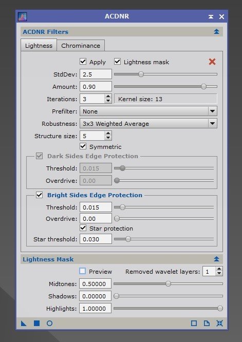
ACDNR panel set up for Ha

Ha before ACDNR
Ha after ACDNR
Final L image based on the Ha image.
9. Create Color Image
Run the SHO-AIP script with new Nonlinear images to create the first color image.

Lum, Red Green, and Blue Linear images ready for combination.

The SHO-AIP Script panel and the settings used to create the initial LRGB linear image.

The initial LRGB image.
11. Initial Process of the Color Image
FInish Processing the Linear Color image
Run DBE to remove any color gradients. Use subtraction and custom sampling selection.
Run PCC to calibrate color. See panel image for parameters used
Run EZ-Denoise on the image
Convert image to Nonlinear
Select background sky reference and create a preview for it
Run MaskedStretch using the preview of each image for the background reference.
Run CT and adjust the tone scale to get a good-looking image.
FInal CT run.
Inject L image into LRGB image using LRGBCombination process.
Use CT to adjust tone scale and color sat.
Create Star masks to correct star images
Use the ColorMask script to create a mask of Magent -adjust with HT to get magenta-blue rings around stars
Apply this and use CT to reduce color curves and sat to reduce rings
Use StarNet++ to creat a starmask. Use CT to reduce color and increase the brightness and size of stars
Apply mask and use CT to adjust star colors
Use ACDNR to Denoise image.
Lightness: Use lightness mask, Std dev of 4.0
Chrominance: Use lightness mask and std dev of 6
Create a range mask to isolate the background sky
I discovered at this point that the background sky had a speckle noise that must be a residual from one of the Denoise operations. I used the range mask to protect the stars and then applied an MLT operation with the first layer removed to clean this up.
EZ-StarReduction with default values and Adam Block method.

PCC panel set up
PCC Regression Fit

After PCC Application.

Linear LRGB image befor EZ-Denoise
Linear LRGB Image after EZ-Denoise run
LRGB Image after Masked Stretch (click to enlarge)
LRGB Image after MaskedStretch and CT adjust (click to enlarge)
LHaRGB Nonlinear image (click ot enlarge)
Magenta Star Mask ring image created with ColorMask and HT adjustments. THis was used to cleanup the stars a bit (click to enlarge)
Starmask created with Starnett++ and then adjusted with CT to make it neutral and boosted in size. This was used to fix the star color that was overly blue.

Range Mask - this was used to clean up the background sky.
This is the final LHaRGB image sent to PS for final touches.
16. Save images as Tiff and Move to Photoshop
In Photoshop:
Use Camera Raw Filter to adjust Global Clarity, Texture, and Color Mix
Use StarShrink filter to reduce large stars radius 35 strength 6, sharpness -1
Use StarShrink filter to reduce small stars radius 2, strength 6, sharpness -1
Use Topaz AI Denoise to reduce noise and sharpen things further
Using Lasso with a father of 150 pixels, select dark regions, and other regions of interesting detail and boost clarity and curves.
Some bright stars had circular regions of neutrality around the star images. I used the healing brush to fix some stars where this was more noticeable
Use the color mixer to adjust hue and saturations.
Add watermarks
Export Clear, Watermarked, and Web-sized Jpegs.

The image before Topaz AI Denoise applied.

After Topaz AI Denoise applied.
And this is the final image….
Adding the next generation ZWO ASI2600MM-Pro camera and ZWO EFW 7x36 II EFW to the platform…