Comparison of Tree Biomass Modeling Approaches for Larch (Larix olgensis Henry) Trees in Northeast China

Abstract

Accurate quantification of tree biomass is critical and essential for calculating carbon storage, as well as for studying climate change, forest health, forest productivity, nutrient cycling, etc. Tree biomass is typically estimated using statistical models. Although various biomass models have been developed thus far, most of them lack a detailed investigation of the additivity properties of biomass components and inherent correlations among the components and aboveground biomass. This study compared the nonadditive and additive biomass models for larch (Larix olgensis Henry) trees in Northeast China. For the nonadditive models, the base model (BM) and mixed effects model (MEM) separately fit the aboveground and component biomass, and they ignore the inherent correlation between the aboveground and component biomass of the same tree sample. For the additive models, two aggregated model systems with one (AMS1) and no constraints (AMS2) and two disaggregated model systems without (DMS1) and with an aboveground biomass model (DMS2) were fitted simultaneously by weighted nonlinear seemingly unrelated regression (NSUR) and applied to ensure additivity properties. Following this, the six biomass modeling approaches were compared to improve the prediction accuracy of these models. The results showed that the MEM with random effects had better model fitting and performance than the BM, AMS1, AMS2, DMS1, and DMS2; however, when no subsample was available to calculate random effects, AMS1, AMS2, DMS1, and DMS2 could be recommended. There was no single biomass modeling approach to predict biomass that was best for all aboveground and component biomass except for MEM. The overall ranking of models based on the fit and validation statistics obeyed the following order: MEM > DMS1 > AMS2 > AMS1> DMS2 > BM. This article emphasized more on the methodologies and it was expected that the methods could be applied by other researchers to develop similar systems of the biomass models for other species, and to verify the differences between the aggregated and disaggregated model systems. Overall, all biomass models in this study have the benefit of being able to predict aboveground and component biomass for larch trees and to be used to predict biomass of larch plantations in Northeast China.

1. Introduction

Plantation forests typically have high growth rates and thereby absorb large amounts of carbon dioxide and help mitigate global climate change. Larch (Larix olgensis Henry) is an important tree species for afforestation and acquiring commercial timber in Northeast China. This species is the fourth most important in China, and it is used to establish fast growing and high-yielding plantation forests, covering a wide geographical range from the northeast to northern subalpine areas of China [1]. Thus, to calculate plantation productivity and study forest health, fuel, nutrient cycling, accurate quantification of tree biomass for larch is critical and essential [2,3,4,5]. A biomass estimation model constructed by direct measurement data of tree biomass is undoubtedly the most appropriate and accurate method for practical applications [6,7,8,9]. To date, hundreds of biomass models have been developed worldwide, in which the diameter at breast height ($DBH$) is a commonly used and most reliable predictor of aboveground and component biomass [8,10,11,12,13,14,15,16]. In addition, tree height ($H$) can also be used as a predictor. Adding $H$ into biomass quantification can significantly improve model fitting and performance, and it can help explain the potential limitation of intra-species divergence. Many studies have shown that biomass models with both $DBH$ and $H$ parameters can more reliably predict tree biomass [5,7,9,17,18,19,20].

At present, model specifications of developing biomass equations for aboveground and components have evolved from nonadditive models to additive models [7,9,20]. Meanwhile, various model estimation methods have been developed to ensure the additivity property for nonlinear biomass models such as the generalized method of moments (GMM), two-stage nonlinear error-in-variable models (TSEM), and nonlinear seemingly unrelated regression (NSUR) [6,7,21,22]. Nonadditive models separately fit the aboveground and component biomass data, and they ignore the inherent correlation among the aboveground and component biomass of the same sample tree. Thus, the biomass models established fall short of statistical efficiency in parameter estimation and fail to consider the additivity among the aboveground and component biomass [7,23]. For nonadditive models, the base model (BM) fitted by nonlinear ordinary least squares (OLS) is believed to be the most widely used technique on parameter estimation, and it is appropriate for datasets with general structures containing random and independent observations [7,24,25,26]. For hierarchically structured data (e.g., trees within plots), mixed effects models (MEM) are likely to be a better choice; they are characterized by fixed parameters corresponding to population and random parameters corresponding to each subject. Some studies have applied MEM to establish component biomass models [27,28,29].

Thus far, two model structures have been used to achieve additivity of the aboveground and component biomass models. Parresol [30] proposed an aggregation model system (referred to as AMS1), in which a nonlinear model is specified for each component, and these component models for stems, branches, and foliage are aggregated to the aboveground biomass. Other researchers proposed that the aboveground biomass model may not occur in Parresol’s model system, i.e., that Parresol’s model system may only fit the component biomass models, rather than the aboveground and component biomass models (referred to as AMS2) [23,31]. The NSUR methods are often used to simultaneously compute the aboveground and component biomass for the aggregation model system [6,7,23,24,25,26,27]. The aggregation model system has become a standard for developing new biomass models because it can easily ensure additivity among the aboveground and component biomass predictions [16,20,23,31]. Tang et al. [32] proposed a disaggregation model system (referred to as DMS1), in which the aboveground biomass model is first developed, and then, the estimated aboveground biomass is disaggregated into different tree components (e.g., stems, branches, and foliage) based on their proportions in the aboveground biomass. Furthermore, some researchers have developed an extended disaggregation model system (referred to as DMS2), in which the aboveground and component biomass models can be fitted simultaneously [21,22]. The TSEM and NSUR methods are often used to estimate the parameters of the aboveground and component biomass models jointly, and to guarantee the additivity of the aboveground and component biomass [7,21,22]. Several studies have shown that the prediction accuracies of the two fitting methods, TSEM and NSUR, were virtually identical for each component and aboveground biomass. However, the advantage of the NSUR method over the TSEM method lies in the fact that it can be readily implemented by PROC MODEL procedure in SAS version 9.3 and nlsystemfit procedure in R version 3.5.1 [7,21,22,33,34].

We aimed to explore the difference in biomass predictions of the BM, MEM, AMS1, AMS2, DMS1, and DMS2. Therefore, the objectives of our study were: (1) to construct two nonadditive biomass models (i.e., BM and MEM) of each component based on $DBH$ only or both $DBH$ and $H$; (2) to construct four additive biomass models (i.e., AMS1, AMS2, DMS1, and DMS2) based on $D$ only or both $D$ and $H$ with weighted NSUR; (3) to verify the performance of the biomass models with jackknife resampling; and (4) to compare the accuracy of model fitting and performance of the different nonadditive and additive biomass models.

2. Materials and Methods

2.1. Data

Data used in this study are obtained from a large dataset of trees sampled from larch plantation stands in Heilongjiang Province, one of the largest forestry provinces in Northeast China. The sample plots were established in July/August of 2007–2016. A total of 40 plots were selected from 10 sites (Figure 1). Each plot was 20 × 30 m or 30 × 30 m in size. For each of the 40 plots, 1–2 sample trees for each of the dominant, codominant, intermediate, and suppressed types were analyzed, and thus, 5–7 trees were sampled from each plot. In total, the dataset consisted of measurements on 229 larch trees using destructive biomass sampling and included the following parameters: diameter at breast height ($DBH$), total tree height ($H$), green weights of stems, branches and foliage, green weights of the sampled disks, branches, and foliage, and the moisture content of disks, branches, and foliage. The specific biomass determination method including field and laboratory measurements followed similar protocols as Dong et al. [5]. For each sampled tree, the sum of branches, foliage, and stem dry biomass was calculated as the aboveground biomass. A summary of the descriptive statistics for $DBH$ and $H$, as well as the aboveground and component biomass of trees is listed in

Table 1. Descriptive statistics of tree variables for all data.

Tree Variables	N	Min	Max	Mean	Std
$DBH$ (cm)	229	2.0	35.7	17.9	6.9
$H$ (m)	229	3.8	27.0	16.8	5.4
Stem biomass (kg)	229	0.27	510.19	133.37	110.83
Branch biomass (kg)	229	0.10	42.30	11.92	8.89
Foliage biomass (kg)	229	0.07	9.79	3.80	2.11
Aboveground biomass (kg)	229	0.40	561.10	149.08	119.60

. The stem, branch, and foliage biomass of all sample trees as well as their relationships with $DBH$ and $H$ are shown in Figure 2.

2.2. Model Specification and Estimation

2.2.1. Base Model

In general, $DBH$ is used as the first variable in tree biomass models because it is simple and easy to apply. To improve the performance of biomass models, $H$ is the second variable incorporated into the model. According to the data obtained by the visual inspection of stems, branches, and foliage, biomass data can be modeled by a power function with $DBH$ and $H$ (Figure 1). Thus, two BMs were used to establish independent component biomass models. These BMs are given by:

$$W_k=e^{{\beta }_{k0}}DB{H}^{{\beta }_{k1}}+{\epsilon }_k$$

(1)

$$W_k=e^{{\beta }_{k0}}DB{H}^{{\beta }_{k1}}{H}^{{\beta }_{k2}}+{\epsilon }_k$$

(2)

where $W_k$ represents the stem, branch, and foliage biomass in kilograms (k = s, b, and f, for stem, branch, and foliage, respectively); $DBH$ and $H$ represent the diameter at breast height and total tree height, respectively; ${\beta }_{k0}$, ${\beta }_{k1}$, and ${\beta }_{k2}$ represents the model parameters; and ${\epsilon }_k$ is the model error term.

2.2.2. Mixed Effects Model

Considering the structure of biomass data, two MEMs with the sample plots as a random factor can be used to establish independent component biomass models. These MEMs are given by:

$$W_{ik}=e^{{\beta }_{k0}+u_{ik0}}DB{H}^{{\beta }_{k1}+u_{ik1}}+{\epsilon }_{ik}$$

(3)

$$W_{ik}=e^{{\beta }_{k0}+u_{ik0}}DB{H}^{{\beta }_{k1}+u_{ik1}}{H}^{{\beta }_{k2}+u_{ik2}}+{\epsilon }_{ik}$$

(4)

where $u_{ik0}$, $u_{ik1}$, and $u_{ik2}$ are the random effect parameters in ith sample plot ($i=1,2,3\dots ,m$), and ${\epsilon }_{ik}$ is the error term. In the equation, ${\epsilon }_{ik}$ obeyed a normal distribution with zero mean and within sample plot variance and covariance matrix $R$, and $u_{ik}$ of the sample plot random effects ($u_{ik0}$, $u_{ik1}$ and $u_{ik2}$) obeyed a normal distribution with zero mean and sample plot variance and covariance matrix $D$.

2.2.3. Aggregated Model Systems

Aggregated model systems fit the component biomass data simultaneously, which explicates the instinctive correlations among the component biomass of the same sample tree. There are two structures for an aggregated model system, i.e., those with one constraint (AMS1) and those with no constraint (AMS2).

• Aggregated model systems with one constraint

Following the model structure specified in Parresol [30], AMS1 ensures additivity between the tree aboveground biomass and component biomass with one constraint: tree aboveground biomass is equal to the sum of the tree component biomass. The expressions of AMS1 with $DBH$ only and combination of $DBH$, $H$ are given as:

$$\{\begin{array}{c}{W}_s=e^{{\beta }_{s0}}DB{H}^{{\beta }_{s1}}+{\epsilon }_s\\ W_b=e^{{\beta }_{b0}}DB{H}^{{\beta }_{b1}}+{\epsilon }_b\\ W_f=e^{{\beta }_{f0}}DB{H}^{{\beta }_{f1}}+{\epsilon }_f\\ W_a=W_s+W_b+W_f+{\epsilon }_a\end{array}$$

(5)

$$\{\begin{array}{c}{W}_s=e^{{\beta }_{s0}}DB{H}^{{\beta }_{s1}}{H}^{{\beta }_{s2}}+{\epsilon }_s\\ W_b=e^{{\beta }_{b0}}DB{H}^{{\beta }_{b1}}{H}^{{\beta }_{b2}}+{\epsilon }_b\\ W_f=e^{{\beta }_{f0}}DB{H}^{{\beta }_{f1}}{H}^{{\beta }_{f2}}+{\epsilon }_f\\ W_a=W_s+W_b+W_f+{\epsilon }_a\end{array}$$

(6)

where a, s, b, and f denote the aboveground, stem, branch, and foliage, respectively.

• Aggregated model systems with no constraint

Following the model structure specified in Affleck and Diéguez-Aranda [31], the expressions of AMS2 with $DBH$ only and a combination of $DBH$ and $H$ are:

$$\{\begin{array}{c}{W}_s=e^{{\beta }_{s0}}DB{H}^{{\beta }_{s1}}+{\epsilon }_s\\ W_b=e^{{\beta }_{b0}}DB{H}^{{\beta }_{b1}}+{\epsilon }_b\\ W_f=e^{{\beta }_{f0}}DB{H}^{{\beta }_{f1}}+{\epsilon }_f\end{array}$$

(7)

$$\{\begin{array}{c}{W}_s=e^{{\beta }_{s0}}DB{H}^{{\beta }_{s1}}{H}^{{\beta }_{s2}}+{\epsilon }_s\\ W_b=e^{{\beta }_{b0}}DB{H}^{{\beta }_{b1}}{H}^{{\beta }_{b2}}+{\epsilon }_b\\ W_f=e^{{\beta }_{f0}}DB{H}^{{\beta }_{f1}}{H}^{{\beta }_{f2}}+{\epsilon }_f\end{array}$$

(8)

2.2.4. Disaggregated Model Systems

Disaggregated model systems can ensure biomass additivity by directly partitioning tree aboveground biomass into three components ($W_s, W_b, \mathrm{and} W_f$) in this study. There are also two structures for the disaggregated model systems, i.e., those without an aboveground biomass model (DMS1) and those with an aboveground biomass model (DMS2).

• Disaggregated model systems without an aboveground biomass model

For DMS1, the given tree aboveground biomass (${\hat{W}}_{a-DBH} \mathrm{and} {\hat{W}}_{a-DBH,H}$) are from the fitted model ${\hat{W}}_{a-DBH}=e^{{\hat{\beta }}_{a0}}DB{H}^{{\hat{\beta }}_{a1}}$ and ${\hat{W}}_{a-DBH,H}=e^{{\hat{\beta }}_{a0}}DB{H}^{{\hat{\beta }}_{a1}}{H}^{{\hat{\beta }}_{a2}}$, respectively. The expressions of DMS1 with $DBH$ only and a combination of $DBH$ and $H$ are as follows:

$$\{\begin{array}{l}\begin{array}{l}{W}_s=\frac{e^{{\beta }_{s0}}DB{H}^{{\beta }_{s1}}}{e^{{\beta }_{s0}}DB{H}^{{\beta }_{s1}}+{\beta }_{b0}DB{H}^{{\beta }_{b1}}+e^{{\beta }_{f0}}DB{H}^{{\beta }_{f1}}}\times {\hat{W}}_{a-DBH}+{\epsilon }_s\\ \hspace{1em}\hspace{1em}\hspace{1em} =\frac{1}{1+{\alpha }_{0}DB{H}^{{\alpha }_1}+{\gamma }_{0}DB{H}^{{\gamma }_1}}\times {\hat{W}}_{a-DBH}+{\epsilon }_s\end{array}\\ \begin{array}{l}{W}_b=\frac{e^{{\beta }_{b0}}DB{H}^{{\beta }_{b1}}}{e^{{\beta }_{s0}}DB{H}^{{\beta }_{s1}}+e^{{\beta }_{b0}}DB{H}^{{\beta }_{b1}}+e^{{\beta }_{f0}}DB{H}^{{\beta }_{f1}}}\times {\hat{W}}_{a-DBH}+{\epsilon }_b\\ \hspace{1em}\hspace{1em}\hspace{1em} =\frac{{\alpha }_{0}DB{H}^{{\alpha }_1}}{1+{\alpha }_{0}DB{H}^{{\alpha }_1}+{\gamma }_{0}DB{H}^{{\gamma }_1}}\times {\hat{W}}_{a-DBH}+{\epsilon }_b\end{array}\\ \begin{array}{l}{W}_f=\frac{e^{{\beta }_{f0}}DB{H}^{{\beta }_{f1}}}{e^{{\beta }_{s0}}DB{H}^{{\beta }_{s1}}+e^{{\beta }_{b0}}DB{H}^{{\beta }_{b1}}+e^{{\beta }_{f0}}DB{H}^{{\beta }_{f1}}}\times {\hat{W}}_{a-DBH}+{\epsilon }_f\\ \hspace{1em}\hspace{1em}\hspace{1em} =\frac{{\gamma }_{0}DB{H}^{{\gamma }_1}}{1+{\alpha }_{0}DB{H}^{{\alpha }_1}+{\gamma }_{0}DB{H}^{{\gamma }_1}}\times {\hat{W}}_{a-DBH}+{\epsilon }_f\end{array}\end{array}$$

(9)

where $\frac{{\beta }_{b0}}{{\beta }_{s0}}={\alpha }_0$, $\frac{{\beta }_{b1}}{{\beta }_{s1}}={\alpha }_1$, $\frac{{\beta }_{f0}}{{\beta }_{s0}}={\gamma }_0$, and $\frac{{\beta }_{f1}}{{\beta }_{s1}}={\gamma }_1$ are model parameters to be estimated.

$$\{\begin{array}{l}\begin{array}{l}{W}_s=\frac{e^{{\beta }_{s0}}DB{H}^{{\beta }_{s1}}{H}^{{\beta }_{s2}}}{e^{{\beta }_{s0}}DB{H}^{{\beta }_{s1}}{H}^{{\beta }_{s2}}+e^{{\beta }_{b0}}DB{H}^{{\beta }_{b1}}{H}^{{\beta }_{b2}}+e^{{\beta }_{f0}}DB{H}^{{\beta }_{f1}}{H}^{{\beta }_{f2}}}\times {\hat{W}}_{a-DBH,H}+{\epsilon }_s\\ \hspace{1em}\hspace{1em}\hspace{1em}\hspace{1em} =\frac{1}{1+{\alpha }_{0}DB{H}^{{\alpha }_1}{H}^{{\alpha }_2}+{\gamma }_{0}DB{H}^{{\gamma }_1{H}^{{\gamma }_2}}}\times {\hat{W}}_{a-DBH,H}+{\epsilon }_s\end{array}\\ \begin{array}{l}{W}_b=\frac{e^{{\beta }_{b0}}DB{H}^{{\beta }_{b1}}}{e^{{\beta }_{s0}}DB{H}^{{\beta }_{s1}}{H}^{{\beta }_{s2}}+e^{{\beta }_{b0}}DB{H}^{{\beta }_{b1}}{H}^{{\beta }_{b2}}+e^{{\beta }_{f0}}DB{H}^{{\beta }_{f1}}{H}^{{\beta }_{f2}}}\times {\hat{W}}_{a-DBH,H}+{\epsilon }_b\\ \hspace{1em}\hspace{1em}\hspace{1em}\hspace{1em} =\frac{{\alpha }_{0}DB{H}^{{\alpha }_1}{H}^{{\alpha }_2}}{1+{\alpha }_{0}DB{H}^{{\alpha }_1}{H}^{{\alpha }_2}+{\gamma }_{0}DB{H}^{{\gamma }_1}{H}^{{\gamma }_2}}\times {\hat{W}}_{a-DBH,H}+{\epsilon }_b\end{array}\\ \begin{array}{l}{W}_f=\frac{e^{{\beta }_{f0}}DB{H}^{{\beta }_{f1}}}{e^{{\beta }_{s0}}DB{H}^{{\beta }_{s1}}{H}^{{\beta }_{s2}}+e^{{\beta }_{b0}}DB{H}^{{\beta }_{b1}}{H}^{{\beta }_{b2}}+e^{{\beta }_{f0}}DB{H}^{{\beta }_{f1}}{H}^{{\beta }_{f2}}}\times {\hat{W}}_{a-DBH,H}+{\epsilon }_f\\ \hspace{1em}\hspace{1em}\hspace{1em}\hspace{1em} =\frac{{\gamma }_{0}DB{H}^{{\gamma }_1}{H}^{{\gamma }_2}}{1+{\alpha }_{0}DB{H}^{{\alpha }_1}{H}^{{\alpha }_2}+{\gamma }_{0}DB{H}^{{\gamma }_1}{H}^{{\gamma }_2}}\times {\hat{W}}_{a-DBH,H}+{\epsilon }_f\end{array}\end{array}$$

(10)

where $\frac{{\beta }_{b2}}{{\beta }_{s2}}={\alpha }_2$, and $\frac{{\beta }_{f2}}{{\beta }_{s2}}={\gamma }_2$ are model parameters to be estimated.

• Disaggregated model systems with an aboveground biomass model

For DMS2, the tree aboveground biomass model ($W_{a-DBH} \mathrm{and} W_{a-DBH,H}$) and component biomass models were fitted simultaneously. The expressions of DMS2 with $DBH$ only and a combination of $DBH$ and $H$ are as follows:

$$\{\begin{array}{l}\begin{array}{l}{W}_s=\frac{e^{{\beta }_{s0}}DB{H}^{{\beta }_{s1}}}{e^{{\beta }_{s0}}DB{H}^{{\beta }_{s1}}+e^{{\beta }_{b0}}DB{H}^{{\beta }_{b1}}+e^{{\beta }_{f0}}DB{H}^{{\beta }_{f1}}}\times W_{a-DBH}+{\epsilon }_s\\ \hspace{1em}\hspace{1em}\hspace{1em} =\frac{1}{1+{\alpha }_{0}DB{H}^{{\alpha }_1}+{\gamma }_{0}DB{H}^{{\gamma }_1}}\times W_{a-DBH}+{\epsilon }_s\end{array}\\ \begin{array}{l}{W}_b=\frac{e^{{\beta }_{b0}}DB{H}^{{\beta }_{b1}}}{e^{{\beta }_{s0}}DB{H}^{{\beta }_{s1}}+e^{{\beta }_{b0}}DB{H}^{{\beta }_{b1}}+e^{{\beta }_{f0}}DB{H}^{{\beta }_{f1}}}\times W_{a-DBH}+{\epsilon }_b\\ \hspace{1em}\hspace{1em}\hspace{1em} =\frac{{\alpha }_{0}DB{H}^{{\alpha }_1}}{1+{\alpha }_{0}DB{H}^{{\alpha }_1}+{\gamma }_{0}DB{H}^{{\gamma }_1}}\times W_{a-DBH}+{\epsilon }_b\end{array}\\ \begin{array}{l}{W}_f=\frac{e^{{\beta }_{f0}}DB{H}^{{\beta }_{f1}}}{e^{{\beta }_{s0}}DB{H}^{{\beta }_{s1}}+e^{{\beta }_{b0}}DB{H}^{{\beta }_{b1}}+e^{{\beta }_{f0}}DB{H}^{{\beta }_{f1}}}\times W_{a-DBH}+{\epsilon }_f\\ \hspace{1em}\hspace{1em}\hspace{1em} =\frac{{\beta }_{0}DB{H}^{{\beta }_1}}{1+{\alpha }_{0}DB{H}^{{\alpha }_1}+{\gamma }_{0}DB{H}^{{\gamma }_1}}\times W_{a-DBH}+{\epsilon }_f\\ \hspace{1em}\hspace{1em}\hspace{1em}\hspace{1em}\hspace{1em} W_{a-DBH}=e^{{\beta }_{a0}}DB{H}^{{\beta }_{a1}}+{\epsilon }_a\end{array}\end{array}$$

(11)

$$\{\begin{array}{l}\begin{array}{l}{W}_s=\frac{e^{{\beta }_{s0}}DB{H}^{{\beta }_{s1}}{H}^{{\beta }_{s2}}}{e^{{\beta }_{s0}}DB{H}^{{\beta }_{s1}}{H}^{{\beta }_{s2}}+e^{{\beta }_{b0}}DB{H}^{{\beta }_{b1}}{H}^{{\beta }_{b2}}+e^{{\beta }_{f0}}DB{H}^{{\beta }_{f1}}{H}^{{\beta }_{f2}}}\times W_{a-DBH,H}+{\epsilon }_s\\ \hspace{1em}\hspace{1em}\hspace{1em}\hspace{1em} =\frac{1}{1+{\alpha }_{0}DB{H}^{{\alpha }_1}{H}^{{\alpha }_2}+{\gamma }_{0}DB{H}^{{\gamma }_1{H}^{{\gamma }_2}}}\times W_{a-DBH,H}+{\epsilon }_s\end{array}\\ \begin{array}{l}{W}_b=\frac{e^{{\beta }_{b0}}DB{H}^{{\beta }_{b1}}}{e^{{\beta }_{s0}}DB{H}^{{\beta }_{s1}}{H}^{{\beta }_{s2}}+e^{{\beta }_{b0}}DB{H}^{{\beta }_{b1}}{H}^{{\beta }_{b2}}+e^{{\beta }_{f0}}DB{H}^{{\beta }_{f1}}{H}^{{\beta }_{f2}}}\times W_{a-DBH,H}+{\epsilon }_b\\ \hspace{1em}\hspace{1em}\hspace{1em}\hspace{1em} =\frac{{\alpha }_{0}DB{H}^{{\alpha }_1}{H}^{{\alpha }_2}}{1+{\alpha }_{0}DB{H}^{{\alpha }_1}{H}^{{\alpha }_2}+{\gamma }_{0}DB{H}^{{\gamma }_1}{H}^{{\gamma }_2}}\times W_{a-DBH,H}+{\epsilon }_b\end{array}\\ \begin{array}{l}{W}_f=\frac{e^{{\beta }_{f0}}DB{H}^{{\beta }_{f1}}}{e^{{\beta }_{s0}}DB{H}^{{\beta }_{s1}}{H}^{{\beta }_{s2}}+e^{{\beta }_{b0}}DB{H}^{{\beta }_{b1}}{H}^{{\beta }_{b2}}+e^{{\beta }_{f0}}DB{H}^{{\beta }_{f1}}{H}^{{\beta }_{f2}}}\times W_{a-DBH,H}+{\epsilon }_f\\ \hspace{1em}\hspace{1em}\hspace{1em}\hspace{1em} =\frac{{\gamma }_{0}DB{H}^{{\gamma }_1}{H}^{{\gamma }_2}}{1+{\alpha }_{0}DB{H}^{{\alpha }_1}{H}^{{\alpha }_2}+{\gamma }_{0}DB{H}^{{\gamma }_1}{H}^{{\gamma }_2}}\times W_{a-DBH,H}+{\epsilon }_f\\ \hspace{1em}\hspace{1em}\hspace{1em}\hspace{1em}\hspace{1em}\hspace{1em}\hspace{1em}{W}_{a-DBH}=e^{{\beta }_{a0}}DB{H}^{{\beta }_{a1}}{H}^{{\beta }_{a2}}+{\epsilon }_a\end{array}\end{array}$$

(12)

2.2.5. Parameter Estimation Methods

In our study, the model parameters in the BM and MEM were estimated using nonlinear ordinary least squares (OLS) and restricted maximum likelihood (REML) methods, respectively. For AMS1, AMS2, DMS1, and DMS2, the model parameters were estimated using nonlinear seemingly unrelated regression (NSUR). More detailed information on the theory and algorithm of the three methods can be found in the literature [7,21,22,23].

All the above models were fitted using different procedures, such as PROC NLIN, PROC NLMIXED, and PROC MODEL in SAS 9.3 software [33].

2.2.6. Weighting Function for Heteroscedasticity

Because of the heteroscedasticity in the model residuals shown by the tree biomass data, to correct the heteroscedasticity of variance, a power variance function of the following equation $\mathrm{var}({\epsilon }_{ik})={\sigma }^2{\hat{W}}_{ik}^{2\varphi }$ was used in the tree biomass models, where ${\epsilon }_{ik}$ is the mixed model residual, $\varphi$ is a parameter to be estimated, ${\hat{W}}_{ik}$ is the estimated biomass of $k$ component of each tree on the ith sample plot using fixed part of the mixed effects model, and ${\sigma }^2$ is a scaling factor for error dispersion [23,35].

2.3. Model Evaluation and Validation

As described above, the six biomass modeling approaches evaluated in this study were: (1) BM, (2) MEM, (3) AMS1, (4) AMS2, (5) DMS1, and (6) DMS2. It is well known that the quality of model fitting does not entirely reflect the quality of future prediction, so that model validation is necessary to assess and evaluate the predictive quality of the different biomass models. Several authors suggest that the most applicable models should be validated using a Jackknifing technique, also known as the “leave-one-out” method or Predicted Sum of Squares (PRESS) [5,7,9]. Thus, in this study, the biomass equations were fitted to the entire dataset (sample trees $N$ of all plots), while model validation was accomplished by Jackknifing technique in which the biomass models were constructed using all but some sample trees of one sampled plot data (fitting data included the sample trees of $m-1$ sample plots), and then the fitted models were used to predict the value of the dependent variable for some sample trees of the excluded sample plot. The model fitting was assessed by two goodness-of-fit statistics (Equations (13) and (14)), and the model performance was evaluated by four model validation statistics of Jackknifing (Equations (15)–(18)) as follows:

The coefficient of determination ($R^2$):

$$R^2=1-\frac{{{\displaystyle \sum }}_{i=1}^m{{\displaystyle \sum }}_{j=1}^{n_j}{(W_{ijk}-{\hat{W}}_{ijk})}^2}{{{\displaystyle \sum }}_{i=1}^m{{\displaystyle \sum }}_{j=1}^{n_j}{(W_{ijk}-{\overline{W}}_k)}^2}$$

(13)

The percent root mean square error (RMSE%):

$$\mathrm{RMSE}\%=\sqrt{\frac{{{\displaystyle \sum }}_{i=1}^m{{\displaystyle \sum }}_{j=1}^{n_j}{\left((W_{ijk}-{\hat{W}}_{ijk)}/W_{ijk}\right)}^2}{{{\displaystyle \sum }}_{i=1}^m{n}_j}}$$

(14)

and the predictive performance (mean prediction error (MPE), mean prediction error percent (MPE%), mean absolute error (MAE), and mean absolute percent error (MAE%) of the tree biomass prediction equation:

$$\mathrm{MPE}=\frac{{{\displaystyle \sum }}_{i=1}^m{{\displaystyle \sum }}_{j=1}^{n_j}\left(W_{ijk}-{\hat{W}}_{ijk,-i}\right)}{{{\displaystyle \sum }}_{i=1}^m{n}_j}$$

(15)

$$\mathrm{MPE}\%=\frac{{{\displaystyle \sum }}_{i=1}^m{{\displaystyle \sum }}_{j=1}^{n_j}(\left(W_{ijk}-{\hat{W}}_{ijk,-i})/{\overline{W}}_k\right)}{{{\displaystyle \sum }}_{i=1}^m{n}_j}$$

(16)

$$\mathrm{MAE}=\frac{{{\displaystyle \sum }}_{i=1}^m{{\displaystyle \sum }}_{j=1}^{n_j}\left|W_{ijk}-{\hat{W}}_{ijk,-i}\right|}{{{\displaystyle \sum }}_{i=1}^m{n}_j}$$

(17)

$$\mathrm{MAE}\%=\frac{{{\displaystyle \sum }}_{i=1}^m{{\displaystyle \sum }}_{j=1}^{n_j}\left|(W_{ijk}-{\hat{W}}_{ijk,-i})/W_{ijk}\right|}{{{\displaystyle \sum }}_{i=1}^m{n}_j}$$

(18)

where $W_{ijk}$ is the observed k (k = s, b, f, and a, represented stem, branch, foliage and aboveground, respectively) component biomass value of jth tree in ith sample plot; ${\hat{W}}_{ijk}$ is the estimated biomass value of jth tree in ith sample plot of the model to which were fitted all the observations of $m$ sample plots; ${\overline{W}}_k$ is the average value of the biomass; ${\hat{W}}_{ijk,-i}$ is the predicted value of the model to which was fitted all the observations of $m-$1 sample plots; $n_j$ was the number of observations in ith sample plot; and m the number of sample plots.

It is important that the parameters of random effects were predicted using the best linear unbiased predictions (BLUPs) method for MEM [36,37]. A vector of random effects parameters of sample plot i was calculated using:

$$u_{ik}=\hat{D}{Z}_{ik}^T{(Z_{ik}\hat{D}{Z}_{ik}^T+\hat{R})}^{-1}{\hat{\epsilon }}_{ik}$$

(19)

where the element of the $Z_{ik}$ matrix was the partial derivative of the nonlinear function with respect to its random parameters; ${\hat{\epsilon }}_{ik}$ was obtained by the difference between the observed and predicted biomass using the model, including only fixed effects; $\hat{D}$ was the variance-covariance matrix estimated in the modelling process; and $\hat{R}$ was the corresponding variance-covariance matrix of within sample plot.

2.4. Comparison of Different Biomass Modeling Approaches

In this study, once the biomass estimate was calculated for each component, the component estimates were summed up to generate the aboveground biomass estimate. We used the six modeling approaches to calculate the biomass of each tree component, and we compared the difference among these modeling approaches using the values of $R^2$, RMSE, MPE, MPE%, MAE, and MAE%.

3. Results

3.1. BM and MEM Based on $DBH$ and $H$

The stem, branch, and foliage biomass equations were fitted independently by weighted OLS and REML. The parameter estimates and their standard errors for the BMs and the MEMs are listed in

Table 2. Parameter estimates and their standard errors (SE) for the base Model (BM) [Equations (1) and (2)] and mixed Effects Model (MEM) [Equations (3) and (4)]. ${\beta }_{k0},{\beta }_{k1}$ and ${\beta }_{k2}$: fixed parameters; $u_{ik0}$, $u_{ik1}$ and $u_{ik2}$: random effect parameters; ${\sigma }_{u_{ik0}}^2$: variance of $u_{ik0}$; ${\sigma }_{u_{ik1}}^2$ variance of $u_{ik1}$;${\sigma }_{u_{ik2}}^2$: variance of $u_{ik2}$ ${\sigma }_{u_{ik0}}{\sigma }_{u_{ik1}}$: covariance of $u_{ik0}$ and $u_{ik1}$; ${\sigma }^2$: residual variance.

Approaches	Model Variables	Components	βk0		βk1		βk2		${\mathit{\sigma }}_{{\mathit{u}}_{\mathit{i}\mathit{k}0}}^2$	${\mathit{\sigma }}_{{\mathit{u}}_{\mathit{i}\mathit{k}1}}^2$	${\mathit{\sigma }}_{{\mathit{u}}_{\mathit{i}\mathit{k}2}}^2$	${\mathit{\sigma }}_{{\mathit{u}}_{\mathit{i}\mathit{k}0}}{\mathit{\sigma }}_{{\mathit{u}}_{\mathit{i}\mathit{k}1}}$	${\mathit{\sigma }}^2$
			Estimate	SE	Estimate	SE	Estimate	SE	Estimate	Estimate	Estimate	Estimate	Estimate
BM	DBH	Stem	−3.6254	0.1094	2.8280	0.0372
		Branch	−3.2894	0.1730	1.9052	0.0601
		Foliage	−2.7397	0.1597	1.3881	0.0536
	DBH and H	Stem	−4.4630	0.0628	1.6982	0.0461	1.4599	0.0580
		Branch	−2.1076	0.2085	2.8131	0.1558	−1.3228	0.1956
		Foliage	−2.2125	0.1843	1.9205	0.1310	−0.7261	0.1594
MEM	DBH	Stem	−2.3110	0.1022	2.3800	0.0325			1.6379				0.2029
		Branch	−4.7310	0.2215	2.4410	0.0696			4.5084	0.1005		−0.6730	0.3069
		Foliage	−3.1880	0.1764	1.5570	0.0615				0.0228			0.4049
	DBH and H	Stem	−4.3494	0.0846	1.7002	0.0454	1.4186	0.0642	0.2189				0.1254
		Branch	−2.7585	0.2648	2.8486	0.1375	−1.1033	0.2003			0.0542		0.3554
		Foliage	−2.3976	0.2155	1.9932	0.1322	−0.7285	0.1714		0.0107			0.4103

. The parameters estimates were significantly different from 0 in each biomass equation (Table 2). For both BM and MEM, the parameter ${\beta }_{i1}$ of $DBH$ was positive for each biomass component, while the parameter ${\beta }_{i2}$ of $H$ was positive for the stem component and negative for the branch and foliage components. These data show that stem biomass increased with an increase in $H$; however, the branch and foliage decreased with an increase of $H$ for the same $DBH$. For BM and MEM, the aboveground biomass should be estimated by summing the estimated stem, branch, and foliage biomass.

3.2. AMS1 and AMS2 Based on $DBH$ and $H$

The parameter estimates of the stem, branch, and foliage biomass models in AMS1 and AMS2 were fitted simultaneously by weighted NSUR and listed in

Table 3. Parameter estimates and their standard errors (SE) for the AMS1 [Equations (5) and (6)] and AMS2 [Equations (7) and (8)].

Approaches	Model Variables	Components	βi0		βi1		βi2
			Estimate	SE	Estimate	SE	Estimate	SE
AMS1	DBH	Stem	−3.7676	0.0946	2.8834	0.0319
		Branch	−3.0780	0.1250	1.8217	0.0443
		Foliage	−2.9308	0.1249	1.4360	0.0421
	DBH and H	Stem	−4.4736	0.058	1.667	0.0431	1.4957	0.0543
		Branch	−2.1082	0.1454	3.0106	0.1194	−1.5347	0.1461
		Foliage	−2.4338	0.1598	2.0931	0.1169	−0.8408	0.1473
AMS2	DBH	Stem	−3.5897	0.1057	2.8216	0.0359
		Branch	−3.1333	0.1587	1.8538	0.0555
		Foliage	−2.757	0.1589	1.3856	0.0533
	DBH and H	Stem	−4.4649	0.0628	1.6980	0.0461	1.4611	0.0579
		Branch	−2.0674	0.2072	2.7545	0.1547	−1.2799	0.1954
		Foliage	−2.1882	0.1858	1.9121	0.1323	−0.7330	0.1613

. The parameters ${\beta }_{i0}$, ${\beta }_{i1}$, and ${\beta }_{i2}$ were highly significant, and their negative or positive prescriptions were consistent with those values in BM and MEM, and they had biological significance. Compared to AMS1, there was no constraint of $W_a=W_r+W_s+W_b+W_f$ and three equations (i.e., stem, branch, and foliage equations) in AMS2. Thus, the aboveground biomass was also estimated by summing the estimated stem, branch, and foliage biomass. For AMS2, a constant 3 × 3 matrix was assumed for cross-correlations among all three equations, and a 4 × 4 matrix was assumed for AMS1.

For example, in this study, there were strong correlations between aboveground and stem biomass, and between branch and foliage components in AMS1 and AMS2 based on $DBH$, as shown in the following two correlation matrices:

$$\begin{array}{cc}AMS1& \begin{array}{cccc}\mathrm{Aboveground}& \mathrm{Stem}& \mathrm{Branch}& \mathrm{Foliage}\end{array}\\ \begin{array}{c}\mathrm{Aboveground}\\ \mathrm{Stem}\\ \mathrm{Branch}\\ \mathrm{Foliage}\end{array}& \left(\begin{array}{cccc}1.0000& 0.9338& -0.0381& 0.0298\\ 0.9338& 1.0000& -0.3315& -0.2073\\ -0.0381& -0.3315& 1.0000& 0.5761\\ 0.0298& -0.2073& 0.5761& 1.0000\end{array}\right)\end{array}$$

$$\begin{array}{cc}AMS2& \begin{array}{ccc}\mathrm{Stem}& \mathrm{Branch}& \mathrm{Foliage}\end{array}\\ \begin{array}{c}\mathrm{Stem}\\ \mathrm{Branch}\\ \mathrm{Foliage}\end{array}& \left(\begin{array}{ccc}1.0000& -0.3439& -0.2246\\ -0.3439& 1.0000& 0.5627\\ -0.2246& 0.5627& 1.0000\end{array}\right)\end{array}$$

3.3. DMS1 and DMS2 Based on $DBH$ and $H$

The only difference between DMS1 and DMS2 lies between the tree aboveground biomass model being fitted independently or simultaneously. The parameter estimates for DMS1 and DMS2 were fitted by weighted NSUR and listed in

Table 4. Parameter estimates and their standard errors (SE) for the DMS1 [Equations (9) and (10)] and DMS2 [Equations (11) and (12)].

Approaches	Model Variables	Parameters	Estimate	SE
DMS1	DBH	α0	1.6051	0.3328
		α1	−0.9811	0.0711
		γ0	2.1940	0.4222
		γ1	−1.4266	0.0641
		βa0	−2.8937	0.0826
		βa1	2.6351	0.0282
	DBH and H	α0	9.5379	2.0289
		α1	1.0793	0.1604
		α2	−2.7155	0.2012
		γ0	8.4438	1.6068
		γ1	0.2201	0.1359
		γ2	−2.1524	0.1678
		βa0	−3.5555	0.0628
		βa1	1.8492	0.0448
		βa2	1.0405	0.0560
DMS2	DBH	α0	3.0795	0.5535
		α1	−1.2101	0.0626
		γ0	3.3838	0.5707
		γ1	−1.5740	0.0569
		βa0	−3.1429	0.0793
		βa1	2.7154	0.0270
	DBH and H	α0	10.7671	1.5583
		α1	1.3375	0.1212
		α2	−3.0285	0.1482
		γ0	7.5777	1.1985
		γ1	0.4091	0.1164
		γ2	−2.3142	0.1482
		βa0	−3.5705	0.0623
		βa1	1.8234	0.0442
		βa2	1.0683	0.0556

. All the other parameter estimates except ${\gamma }_1$ were highly significant in each biomass equation. Similarly, a 3 × 3 and 4 × 4 matrixes for cross-correlations in DMS1 and DMS2 based on $DBH$ are given by:

$$\begin{array}{cc}DMS1& \begin{array}{ccc}\mathrm{Stem}& \mathrm{Branch}& \mathrm{Foliage}\end{array}\\ \begin{array}{c}\mathrm{Stem}\\ \mathrm{Branch}\\ \mathrm{Foliage}\end{array}& \left(\begin{array}{ccc}1.0000& -0.3595& -0.2462\\ -0.3595& 1.0000& 0.5575\\ -0.2462& 0.5575& 1.0000\end{array}\right)\end{array}$$

$$\begin{array}{cc}DMS2& \begin{array}{cccc}\mathrm{Aboveground}& \mathrm{Stem}& \mathrm{Branch}& \mathrm{Foliage}\end{array}\\ \begin{array}{c}\mathrm{Aboveground}\\ \mathrm{Stem}\\ \mathrm{Branch}\\ \mathrm{Foliage}\end{array}& \left(\begin{array}{cccc}1.0000& 0.9438& -0.0759& 0.0209\\ 0.9438& 1.0000& -0.3435& -0.2309\\ -0.0759& -0.3435& 1.0000& 0.5761\\ 0.0209& -0.2309& 0.5761& 1.0000\end{array}\right)\end{array}$$

As with AMS1 and AMS2, there were high correlations between the aboveground and stem biomass, between the branch and foliage components, and weak correlations between the aboveground and branch components and between the aboveground and foliage components.

3.4. Comparison between Different Biomass Modeling Approaches

Table 5. Goodness-of-fit statistics and the parameter of weight functions ($\varphi$) for the biomass models developed using the BM, MEM, AMS1, AMS2, DMS1, and DMS2.

Approaches	Model Variables	Variables	Stem	Branch	Foliage	Aboveground
BM	DBH	R2	0.9291	0.6675	0.7045	0.9420
		RMSE%	22.86	52.63	88.07	16.84
		$\varphi$	1.7666	1.8852	1.3586	-
	DBH and H	R2	0.9738	0.7239	0.7213	0.9764
		RMSE%	11.20	49.53	78.51	10.69
		$\varphi$	1.876	1.7848	1.3512	-
MEM	DBH	R2	0.9757	0.8631	0.8056	0.9773
		RMSE%	12.07	33.14	77.6	11.09
		$\varphi$	1.7666	1.8852	1.3586	-
	DBH and H	R2	0.9839	0.8597	0.7938	0.9844
		RMSE%	9.19	38.11	74.91	8.94
		$\varphi$	1.876	1.7848	1.3512	-
AMS1	DBH	R2	0.9237	0.6307	0.6893	0.9393
		RMSE%	23.33	52.34	78.82	17.01
		$\varphi$	1.7666	1.8852	1.3586	1.7772
	DBH and H	R2	0.9737	0.7151	0.7062	0.9763
		RMSE%	11.22	46.88	66.93	10.52
		$\varphi$	1.876	1.7848	1.3512	1.7866
AMS2	DBH	R2	0.9296	0.6627	0.6996	0.9432
		RMSE%	23.24	53.8	85.75	16.83
		$\varphi$	1.7666	1.8852	1.3586	-
	DBH and H	R2	0.9738	0.7172	0.7202	0.9764
		RMSE%	11.22	49.61	77.59	10.73
		$\varphi$	1.876	1.7848	1.3512	-
DMS1	DBH	R2	0.9349	0.6507	0.7037	0.9478
		RMSE%	24.88	53.74	82.73	27.33
		$\varphi$	1.7666	1.8852	1.3586	1.7772
	DBH and H	R2	0.9744	0.7235	0.7215	0.9769
		RMSE%	12.04	49.48	75.22	18.19
		$\varphi$	1.876	1.7848	1.3512	1.7866
DMS2	DBH	R2	0.9285	0.5986	0.6976	0.9442
		RMSE%	24.78	53.75	81.94	17.73
		$\varphi$	1.7666	1.8852	1.3586	1.7772
	DBH and H	R2	0.9745	0.7121	0.7099	0.9767
		RMSE%	11.76	47.20	68.17	10.81
		$\varphi$	1.876	1.7848	1.3512	1.7866

shows the $R^2$, RMSE%, and weight functions for each biomass equation developed using the six different biomass modeling approaches. The results indicated that a majority of the biomass equations fit the biomass data well, with $R^2$ > 0.70. All models fit the aboveground and stem biomass data best, while small $R^2$ values were observed in the branch and foliage biomass equations. Figure 3 shows the scatterplots of the observed aboveground and component biomass as well as the model predictions by the six biomass modeling approaches. Table 5 and Figure 3 indicated that the MEM with $DBH$ only and combination of $DBH$ and $H$ yielded higher $R^2$ and smaller RMSE% than did the other five biomass modeling approaches, and the addition of $H$ improved the goodness-of-fit for the majority of the aboveground and component biomass equations. The DMS1 and AMS2 produced a slightly larger $R^2$ value for most of the aboveground and component biomass models, compared with AMS1 and DMS2, and had a very close values of $R^2$ and RMSE% for predicting the aboveground and component biomass (Table 5).

Furthermore, we used the jackknifing technique to assess the validity of these biomass models. The model validation statistics were computed and presented in

Table 6. Jackknifing validation of the six biomass modeling approaches.

Approaches	Model Variables	Variables	Stem	Branch	Foliage	Aboveground
BM	DBH	MPE	5.14	1.65	0.11	6.89
		MPE%	3.85	13.85	2.89	4.62
		MAE	20.21	3.58	0.89	19.27
		MAE%	19.15	36.9	26.97	14.92
	DBH and H	MPE	0.93	1.05	0.06	2.04
		MPE%	0.70	8.81	1.58	1.37
		MAE	11.32	3.27	0.88	11.96
		MAE%	8.95	30.42	26.22	8.95
MEM	DBH	MPE	−0.32	0.02	0.01	−0.29
		MPE%	−0.24	0.17	0.26	−0.19
		MAE	10.23	2.16	0.83	10.68
		MAE%	8.80	19.21	24.53	8.02
	DBH and H	MPE	0.35	0.04	0.00	0.39
		MPE%	0.26	0.34	0.09	0.26
		MAE	8.91	2.24	0.75	9.36
		MAE%	7.17	20.34	22.42	6.92
AMS1	DBH	MPE	1.06	2.09	0.27	3.42
		MPE%	0.79	17.54	7.11	2.29
		MAE	20.40	3.72	0.9	19.34
		MAE%	19.31	38.61	29.17	14.84
	DBH and H	MPE	0.90	1.25	0.19	2.35
		MPE%	0.67	10.49	5.00	1.58
		MAE	11.36	3.35	0.90	12.02
		MAE%	8.96	31.24	27.62	8.84
AMS2	DBH	MPE	3.09	1.66	0.20	4.95
		MPE%	2.32	13.93	5.26	3.32
		MAE	20.09	3.58	0.89	19.01
		MAE%	18.52	36.13	27.76	14.38
	DBH and H	MPE	0.75	1.19	0.14	2.08
		MPE%	0.56	9.99	3.68	1.40
		MAE	11.32	3.3	0.88	11.98
		MAE%	8.94	30.74	26.78	8.97
DMS1	DBH	MPE	1.32	1.73	0.19	3.25
		MPE%	0.99	14.52	5.00	2.18
		MAE	19.66	3.6	0.88	18.43
		MAE%	18.69	35.68	27.11	14.15
	DBH and H	MPE	−0.39	1.03	0.11	0.75
		MPE%	−0.29	8.64	2.89	0.50
		MAE	11.35	3.27	0.88	11.83
		MAE%	9.48	30.38	26.53	9.06
DMS2	DBH	MPE	0.53	2.22	0.26	3.01
		MPE%	0.40	18.63	6.84	2.02
		MAE	20.05	3.78	0.88	18.84
		MAE%	21.66	37.58	27.4	15.47
	DBH and H	MPE	1.02	1.26	0.19	2.47
		MPE%	0.76	10.57	5.00	1.66
		MAE	11.3	3.36	0.90	12.02
		MAE%	9.41	32.27	27.81	9.23

, in which MPE and MPE% represented the average prediction error, and MAE and MAE% represented the magnitude of prediction error. The model prediction error varied across the different biomass modeling approaches. Model jackknife statistics indicated the stem biomass models of MEM based $DBH$ and DMS1 based combination of $DBH$ and $H$ slightly overestimated the tree stem biomass (MPE < −0.5 kg and MPE% < −0.3%), and the other biomass models underestimated stem, branch, foliage, and aboveground biomass (MPE > 0.3 kg and MPE% > 0.3%) (Table 6). For all biomass modeling approaches, the average prediction error of the branch biomass was the largest (MAE% was between 19%~39%) and the average prediction error of the aboveground biomass was the smallest (MAE% was between 6%~16%). Biomass models based on a combination of $DBH$ and $H$ seemed preferable to biomass models based on $DBH$ only.

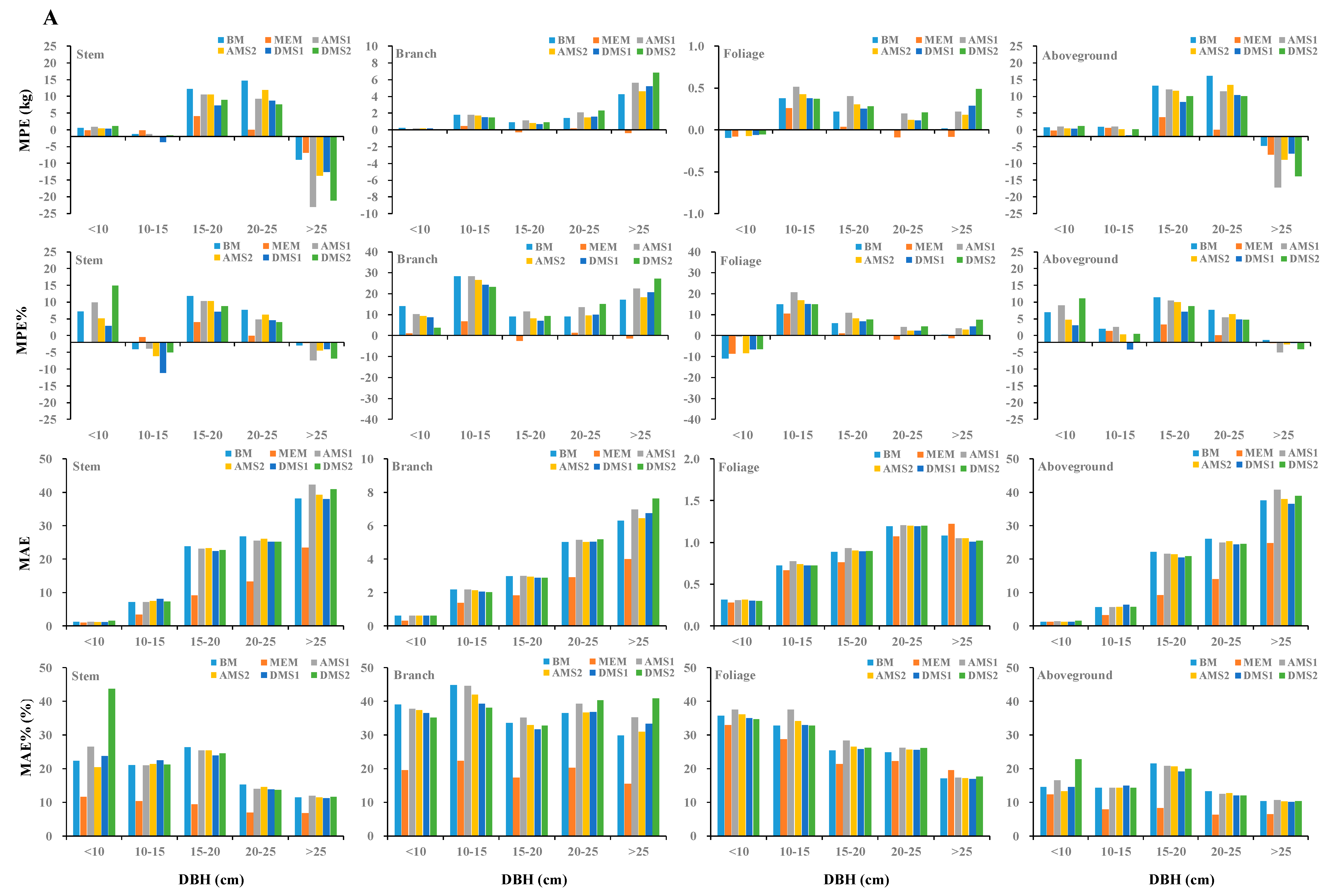
The validation statistics suggested that MEM was better than BM, AMS1, AMS2, DMS1, and DMS2 at predicting the aboveground and component biomass; no significant differences among between BM, AMS1, AMS2, DMS1, and DMS2 were observed (Table 6). To better compare the different biomass modeling approaches, prediction across the diameter classes would be a good method to validate tree biomass models. In this study, the MPE, MPE%, MAE, and MAE% in tree components of different biomass modeling approaches are based on $DBH$ only, and the combination of $DBH$ and $H$ are shown in Figure 4. The figure indicates that the six biomass modeling approaches with $DBH$ only and combination of $DBH$ and $H$ fitted well for the aboveground and component biomass for larch. Furthermore, the MEM did better than the other five biomass modeling approaches for most diameter classes and adding $H$ into biomass models reduced the prediction error in all classes, especially in the largest diameter class ($D$ > 25 cm).

Overall, based on $R^2$, RMSE, MPE, MPE%, MAE, and MAE% for the aboveground and component biomass, the MEM was the best for the aboveground and each component biomass, and the DMS1 was slightly better than BM, AMS1, AMS2, and DMS2 for most component biomass. Compared with the AMS1, AMS2 decreased the most of MPE, MPE%, MAE, and MAE% for aboveground, stem, branch, and foliage biomass, and it would be better for estimating the aggregated models. Similarly, DMS1 was better for estimating the disaggregated models.

4. Discussions

For the selection of biomass model variables, $DBH$ is an indispensable predictor of biomass models. In practice, tree biomass models constructed with only $DBH$ require basic forest inventory data in their application [10,20,38]. Our results showed that $DBH$ was the primary explanatory variable in the component biomass models. This may originate from the intimate correlations between components and tree diameter [7,10,20,39]. However, within the given $DBH$, there is usually some variation among the aboveground and component biomass values, which highlight that it is insufficient to predict the aboveground and component biomass by the biomass model constructed with only $DBH$. Thus, to improve the prediction accuracy of the aboveground and component biomass models, another variable should be added into the biomass model [20]. An increasing number of scholars have often considered $H$ as another commonly used and vital predictor variable to reduce biased estimates of biomass models because tree height usually reflects the site factors [15,18]. In our study, to simulate the biomass allometric relationships for larch trees, $W_k=e^{{\beta }_{k0}}DB{H}^{{\beta }_{k1}}$ and $W_k=e^{{\beta }_{k0}}DB{H}^{{\beta }_{k1}}{H}^{{\beta }_{k2}}$ were selected to construct basic equations. Six biomass modeling approaches were constructed and validated with the jackknifing technique. Our findings were consistent with previous studies, i.e., that a combination of $DBH$ and $H$ significantly improved the prediction accuracy of aboveground and component biomass [6,7,9,40].

Tree biomass models are categorized as nonadditive or additive models. Nonadditive models cannot synchronously consider the aboveground and component biomass data, leading to unequal aboveground biomass. The additive biomass models comprise a desirable characteristic for a system of equations used for the tree biomass prediction, which explicate the instinctive correlations among component biomass of the same sample, and thus, they have a great statistical efficiency [23,30,41]. In this study, we applied six biomass modeling approaches to develop the biomass models. The BM and MEM have separately fitted aboveground and component biomass models, and they did not hold the additivity property for aboveground biomass. Therefore, the sums of the predictions of tree component models were usually larger or smaller than the predictions of the aboveground biomass models, although the differences were small. In contrast, AMS1, AMS2, DMS1, and DMS2 successfully accounted for the correlations among component biomass by a covariance matrix, in which the aboveground biomass prediction was aggregated from the predictions of the tree component models or disaggregated into tree component biomass. Thus, the AMS1, AMS2, DMS1, and DMS2 held the additivity property for the aboveground biomass.

The AMS1 and AMS2 was fitted with independent nonlinear biomass models, in which there is no random effect in each model. The AMS2 contains no constraint, while AMS1 contains one constraint that guarantees that aboveground predictions will be exactly equal to the sum of the biomass prediction of the stem, branch, and foliage component. Our results indicated that both AMS1 and AMS2 fitted the data and performed well in terms of the average prediction errors for aboveground and component biomass predictions. In this study, we demonstrated the differences between AMS1 and AMS2 because of the constraints imposed on the model system. Furthermore, the AMS1 and AMS2 in our study had smaller standard errors of parameters compared to BM, although AMS1, AMS2, and BM possess similar $R^2$, RMSE%, MPE, MPE%, MAE, and MAE%, which was consistent with results from Parresol [30]. In comparison to the BM, the AMS1 and AMS2 accounted for correlations between component biomass and focus on additivity. Therefore, we recommend AMS1 and AMS2 over the BM. In addition, AMS2 was indeed better for predicting the aboveground and component biomass than AMS1, even though AMS1 actually uses aboveground biomass model as a dependent equation. These data are in accordance with those from Zhao et al. [23]. Thus, the AMS2 is more suitable to construct the biomass models for aggregated model systems.

Both DMS1 and DMS2 maintained the properties of additivity for the aboveground and component biomass. In our study, the prediction accuracy of the aboveground and each component biomass model using DMS1 were higher than those from using DMS2. This is likely because disaggregated model systems depend on the aboveground biomass model, which is commonly thought to be the most accurate among the aboveground and component biomass models [7]. Although DMS1 was slightly superior to AMS2, the advantage of AMS2 over DMS1 lies in the fact that it has been successfully implemented for individual biomass estimation, and that it is more maneuverable in practical applications.

The results in Table 5, Table 6, and Figure 4 show that the biomass models were obviously improved on the fit and validation statistics after including the sample plot as a random effect into MEM. Consequently, the MEM in the above six approaches selected is probably more suitable for this study. Many studies have shown that biotic factors (e.g., $DBH$, $H$) and abiotic factors (e.g., origin, site, and climate) affect the biomass prediction accuracy [7,9,21,23,27]. The random effect “plot” added into the MEM could relate to climatic factors or site factors. In other words, BM, AMS1, AMS2, DMS1, and DMS2 consider the influence of biotic factors only, the MEM also takes abiotic factors into account, making it the most efficient among the six biomass modeling approaches. In fact, the fixed effects parameters in MEM has larger standard errors among all six approaches (Table 2). Thus, when a subsample of biomass is available to predict the random effects, the MEM is more efficient than the other five biomass modeling approaches. However, if the subsample is available, the MEM without the random effects would obtain less efficient estimates. At this point, we would recommend the use of the AMS2 or DMS1.

5. Conclusions

We developed six biomass modeling approaches based on $DBH$ only and a combination of $DBH$, $H$ for larch trees occupying a relatively large geographical area in Northeast China. The BM, MEM, AMS1, AMS2, DMS1, and DMS2 separately fitted the component biomass. We compared the six biomass modeling approaches based on $R^2$, RMSE%, MPE, MPE%, MAE, and MAE%. Our results indicated the MEM with random effects had better $R^2$, RMSE%, MPE, MPE%, MAE, and MAE% than the BM, AMS1, AMS2, DMS1, and DMS2, and thus, it was selected as the most suitable for this study. However, when no subsample is available to calculate the random effects, the aggregated and disaggregated model systems are recommended because these model systems had better fitting and smaller standard errors of the parameters than the BM did; furthermore, they also accounted for correlations among the aboveground and component biomass. Between the aggregated model systems, AMS2 was better for predicting the aboveground and component biomass than AMS1; DMS1 was better than DMS2. Furthermore, with regard to biomass estimation, there was no single model or system to predict biomass that was best for the aboveground and component biomass. For this study, the overall ranking based on the fit and validation statistics obeyed the following order: MEM > DMS1 > AMS2 > AMS1 > DMS2 > BM.

Our future work will aim to use conifer and deciduous tree species to verify the differences between the aggregated and disaggregated model systems, as well as compare the differences between AMS1 against AMS2, or DMS1 against DMS2. The biomass models described in our study are useful tools for the prediction of the aboveground and component biomass for larch trees in different locations and supply basic information to the Chinese National Forest Inventory.

References

- State Forestry and Grassland Administration. The Ninth Forest Resource Survey Report (2014–2018); China forestry press: Beijing, China, 2019; p. 451. (In Chinese) [Google Scholar]
- Konôpka, B.; Pajtík, J.; Noguchi, K.; Lukac, M. Replacing Norway spruce with European beech: A comparison of biomass and net primary production patterns in young stands. For. Ecol. Manag. 2013, 302, 185–192. [Google Scholar] [CrossRef]
- Houghton, R.A. Aboveground Forest Biomass and the Global Carbon Balance. Glob. Chang. Biol. 2005, 11, 945–958. [Google Scholar] [CrossRef]
- Zeng, W.S.; Duo, H.; Lei, X.; Chen, X.; Wang, X.; Pu, Y.; Zou, W. Individual tree biomass equations and growth models sensitive to climate variables forLarixspp in China. Eur. J. For. Res. 2017, 136, 233–249. [Google Scholar] [CrossRef]
- Dong, L.H.; Zhang, L.J.; Li, F.R. Developing Two additive biomass equations for three coniferous plantation species in Northeast China. Forests 2016, 7, 136. [Google Scholar] [CrossRef] [Green Version]
- Bi, H.; Turner, J.; Lambert, M.J. Additive biomass equations for native eucalypt forest trees of temperate Australia. Trees 2004, 18, 467–479. [Google Scholar] [CrossRef]
- Dong, L.; Zhang, L.; Li, F. A Three-Step Proportional Weighting System of Nonlinear Biomass Equations. For. Sci. 2015, 61, 35–45. [Google Scholar] [CrossRef]
- Weiskittel, A.R.; MacFarlane, D.W.; Radtke, P.J.; Affleck, D.L.R.; Temesgen, H.; Woodall, C.W.; Westfall, J.A.; Coulston, J.W. A Call to Improve Methods for Estimating Tree Biomass for Regional and National Assessments. J. For. 2015, 113, 414–424. [Google Scholar] [CrossRef] [Green Version]
- Zhao, D.; Kane, M.; Markewitz, D.; Teskey, R.; Clutter, M. Additive Tree Biomass Equations for Midrotation Loblolly Pine Plantations. For. Sci. 2015, 61, 613–623. [Google Scholar] [CrossRef] [Green Version]
- Wang, C. Biomass allometric equations for 10 co-occurring tree species in Chinese temperate forests. For. Ecol. Manag. 2006, 222, 9–16. [Google Scholar] [CrossRef]
- Henry, M.; Picard, N.; Trotta, C.; Manlay, R.J.; Valentini, R.; Bernoux, M.; Saint-Andre, L. Estimating Tree Biomass of Sub-Saharan African Forests: A Review of Available Allometric Equations. Silva Fenn. 2011, 45, 477–569. [Google Scholar] [CrossRef] [Green Version]
- Chave, J.; Rejou-Mechain, M.; Burquez, A.; Chidumayo, E.; Colgan, M.S.; Delitti, W.B.C.; Duque, A.; Eid, T.; Fearnside, P.M.; Goodman, R.C.; et al. Improved allometric models to estimate the aboveground biomass of tropical trees. Glob. Chang. Biol. 2014, 20, 3177–3190. [Google Scholar] [CrossRef]
- Sileshi, W.G. A critical review of forest biomass estimation models, common mistakes and corrective measures. For. Ecol. Manag. 2014, 329, 237–254. [Google Scholar] [CrossRef]
- Temesgen, H.; Affleck, D.; Poudel, K.; Gray, A.; Sessions, J. A review of the challenges and opportunities in estimating above ground forest biomass using tree-level models. Scand. J. For. Res. 2015, 30, 326–335. [Google Scholar] [CrossRef]
- Yuen, J.Q.; Fung, T.; Ziegler, A.D. Review of allometric equations for major land covers in SE Asia: Uncertainty and implications for above- and below-ground carbon estimates. For. Ecol. Manag. 2016, 360, 323–340. [Google Scholar] [CrossRef]
- Wang, X.; Zhao, D.; Liu, G.; Yang, C.; Teskey, R.O. Additive tree biomass equations for Betula platyphylla Suk plantations in Northeast China. Ann. For. Sci. 2018, 75, 60. [Google Scholar] [CrossRef] [Green Version]
- Kralicek, K.; Huy, B.; Poudel, K.P.; Temesgen, H.; Salas, C. Simultaneous estimation of above- and below-ground biomass in tropical forests of Viet Nam. For. Ecol. Manag. 2017, 390, 147–156. [Google Scholar] [CrossRef]
- Bi, H.; Murphy, S.; Volkova, L.; Weston, C.; Fairman, T.; Li, Y.; Law, R.; Norris, J.; Lei, X.; Caccamo, G. Additive biomass equations based on complete weighing of sample trees for open eucalypt forest species in south-eastern Australia. For. Ecol. Manag. 2015, 349, 106–121. [Google Scholar] [CrossRef]
- Meng, S.; Liu, Q.; Zhou, G.; Jia, Q.; Zhuang, H.; Zhou, H. Aboveground tree additive biomass equations for two dominant deciduous tree species in Daxing’anling, northernmost China. J. For. Res. 2017, 22, 233–240. [Google Scholar] [CrossRef]
- Dong, L.; Zhang, L.; Li, F. Additive Biomass Equations Based on Different Dendrometric Variables for Two Dominant Species (Larix gmelini Rupr. and Betula platyphylla Suk.) in Natural Forests in the Eastern Daxing’an Mountains, Northeast China. Forests 2018, 9, 261. [Google Scholar] [CrossRef] [Green Version]
- Fu, L.; Lei, Y.; Wang, G.; Bi, H.; Tang, S.; Song, X. Comparison of seemingly unrelated regressions with error-in-variable models for developing a system of nonlinear additive biomass equations. Trees 2016, 30, 839–857. [Google Scholar] [CrossRef]
- Lei, Y.; Fu, L.; Affleck, D.L.R.; Nelson, A.S.; Shen, C.; Wang, M.; Zheng, J.; Ye, Q.; Yang, G. Additivity of nonlinear tree crown width models: Aggregated and disaggregated model structures using nonlinear simultaneous equations. For. Ecol. Manage. 2018, 427, 372–382. [Google Scholar] [CrossRef]
- Zhao, D.; Westfall, J.; Coulston, J.W.; Lynch, T.B.; Bullock, B.P.; Montes, C.R. Additive biomass equations for slash pine trees: Comparing three modeling approaches. Can. J. For. Res. 2019, 49, 27–40. [Google Scholar] [CrossRef]
- Zhou, X.; Brandle, J.R.; Schoeneberger, M.M.; Awada, T. Developing above-ground woody biomass equations for open-grown, multiple-stemmed tree species: Shelterbelt-grown Russian-olive. Ecol. Model. 2007, 202, 311–323. [Google Scholar] [CrossRef] [Green Version]
- Koala, J.; Sawadogo, L.; Savadogo, P.; Aynekulu, E.; Heiskanen, J.; Said, M. Allometric equations for below-ground biomass of four key woody species in West African savanna-woodlands. Silva Fenn. 2017, 51, 1631. [Google Scholar] [CrossRef] [Green Version]
- Kenzo, T.; Himmapan, W.; Yoneda, R.; Tedsorn, N.; Vacharangkura, T.; Hitsuma, G.; Noda, I. General estimation models for above- and below-ground biomass of teak (Tectona grandis) plantations in Thailand. For. Ecol. Manag. 2020, 457, 117701. [Google Scholar] [CrossRef]
- Zheng, C.; Mason, E.G.; Jia, L.; Wei, S.; Sun, C.; Duan, J. A single-tree additive biomass model of Quercus variabilis Blume forests in North China. Trees 2015, 29, 705–716. [Google Scholar] [CrossRef] [Green Version]
- Njana, M.A.; Bollandsas, O.M.; Eid, T.; Zahabu, E.; Malimbwi, R.E. Above- and belowground tree biomass models for three mangrove species in Tanzania: A nonlinear mixed effects modelling approach. Ann. For. Sci. 2016, 73, 353–369. [Google Scholar] [CrossRef] [Green Version]
- Chen, D.; Huang, X.; Zhang, S.; Sun, X. Biomass Modeling of Larch (Larix spp.) Plantations in China Based on the Mixed Model, Dummy Variable Model, and Bayesian Hierarchical Model. Forests 2017, 8, 268. [Google Scholar] [CrossRef] [Green Version]
- Parresol, B. Additivity of nonlinear biomass equations. Can. J. For. Res. 2001, 31, 865–878. [Google Scholar] [CrossRef]
- Affleck, D.L.R.; Dieguez-Aranda, U. Additive Nonlinear Biomass Equations: A Likelihood-Based Approach. For. Sci. 2016, 62, 129–140. [Google Scholar] [CrossRef]
- Tang, S.; Zhang, H.; Xu, H. Study on establish and estimate method of compatible biomass model. Sci. Silvae Sin. 2000, 36, 19–27. [Google Scholar]
- SAS Institute Inc. SAS/ETS® 9.3. User’s Guide; SAS Institute Inc.: Cary, NC, USA, 2011; p. 3302. [Google Scholar]
- R Core Team. R: A Language and Environment for Statistical Computing; R Foundation for Statistical Computing: Vienna, Austria, 2019. [Google Scholar]
- Fu, L.; Sun, H.; Sharma, R.P.; Lei, Y.; Zhang, H.; Tang, S. Nonlinear mixed-effects crown width models for individual trees of Chinese fir (Cunninghamia lanceolata) in south-central China. For. Ecol. Manag. 2013, 302, 210–220. [Google Scholar] [CrossRef]
- Pinheiro, J.C.; Bates, D.M. Mixed-Effects Models in S and S-Plus, 1st ed.; Springer: New York, NY, USA, 2000; p. 528. [Google Scholar]
- Ni, C.; Nigh, G.D. An analysis and comparison of predictors of random parameters demonstrated on planted loblolly pine diameter growth prediction. Forestry 2012, 85, 271–280. [Google Scholar] [CrossRef] [Green Version]
- Jenkins, J.C.; Chojnacky, D.C.; Heath, L.S.; Birdsey, R.A. National-scale biomass estimators for United States tree species. For. Sci. 2003, 49, 12–35. [Google Scholar]
- Kapinga, K.; Syampungani, S.; Kasubika, R.; Yambayamba, A.M.; Shamaoma, H. Species-specific allometric models for estimation of the above-ground carbon stock in miombo woodlands of Copperbelt Province of Zambia. For. Ecol. Manag. 2018, 417, 184–196. [Google Scholar] [CrossRef]
- Ali, A.; Xu, M.S.; Zhao, Y.T.; Zhang, Q.Q.; Zhou, L.L.; Yang, X.D.; Yan, E.R. Allometric biomass equations for shrub and small tree species in subtropical China. Silva Fenn. 2015, 49, 1–10. [Google Scholar] [CrossRef] [Green Version]
- Parresol, B.R. Assessing Tree and Stand Biomass: A Review with Examples and Critical Comparisons. For. Sci. 1999, 45, 573–593. [Google Scholar]
Figure 1.
Geographical position of study area and sampling plots in Heilongjiang Province of Northeast China.
Figure 2.
Relationships between stem, branch, and foliage biomass and diameter at breast height () and tree height ().
Figure 3.
The observed data and model predictions from the six biomass modeling approaches based on and combination of and for stem, branch, foliage, and aboveground biomass.
Figure 4.
Comparison of model performance for the six biomass modeling approaches based on (A) and combination of and (B) across diameter classes by the mean prediction error (MPE), mean prediction error percent (MPE%),mean absolute error (MAE), and mean absolute percent error (MAE%) in aboveground and components biomass.