Article

Estimating Needle and Shoot Inclination Angle Distributions and Projection Functions in Five Larix principis-rupprechtii Plots via Leveled Digital Camera Photography

1
The Academy of Digital China (Fujian), Fuzhou University, Fuzhou 350116, China
2
Key Laboratory of Spatial Data Mining and Information Sharing, Ministry of Education, Fuzhou 350116, China
*
Author to whom correspondence should be addressed.
Forests 2021, 12(1), 30; https://doi.org/10.3390/f12010030
Submission received: 16 August 2020 / Revised: 21 December 2020 / Accepted: 25 December 2020 / Published: 28 December 2020
(This article belongs to the Section Forest Inventory, Modeling and Remote Sensing)

Abstract

:
The leaf inclination angle distribution function is a key determinant that influences radiation penetration through forest canopies. In this study, the needle and shoot inclination angle distributions of five contrasting Larix principis-rupprechtii plots were obtained via the frequently used leveled digital camera photography method. We also developed a quasi-automatic method to derive the needle inclination angles based on photographs obtained using the leveled digital camera photography method and further verified using manual measurements. Then, the variations of shoot and needle inclination angle distributions due to height levels, plots, and observation years were investigated. The results showed that the developed quasi-automatic method is effective in deriving needle inclination angles. The shoot and needle inclination angle distributions at the whole-canopy scale tended to be planophile and exhibited minor variations with plots and observation years. The small variations in the needle inclination angle distributions with height level in the five plots might be caused by contrasting light conditions at different height levels. The whole-canopy and height level needle projection functions also tended to be planophile, and minor needle projection function variations with plots and observation years were observed. We attempted to derive the shoot projection functions of the five plots by using a simple and applicable method and further evaluated the performance of the new method.

1. Introduction

The leaf inclination angle distribution function (LIDF), which is defined as the probability of a leaf element of unit size to have its surface normal within a specified unit solid angle [1,2], is a key determinant influencing radiation penetration through forest canopies [3]. The LIDF is also the fundamental parameter used to derive the leaf projection function (commonly referred to as G ), which is defined as the projection coefficient of the unit foliage area on a plane perpendicular to the viewing direction [2]. This coefficient is required as the key parameter for the indirect estimation of the leaf area index (LAI) using optical methods. Therefore, LIDF and G measurements are essential requirements in the field of forestry.
Although LIDF measurements are required for many forest studies, few reliable and convenient estimation methods (i.e., direct and indirect methods) are available for forest canopies, especially for coniferous forest canopies. For example, although some direct methods have been successfully applied to measure the LIDFs of low-vegetation canopies by using combinations of inclinometers, compasses and rulers [2,4], mechanical arms [5], and 3D digitizers [6,7], they are difficult to apply in tall canopies, such as forest canopies, because they must be in contact with leaves, which are usually distant from the ground instrument and operator. Several indirect methods, including optical methods (e.g., multiband vegetation imaging [8], digital hemispherical photography (DHP) [9,10] and digital cover photography [11,12], leveled digital photography (LDP) [3,13,14,15]), 3D image-processing method [16] and terrestrial laser scanning [17,18,19,20,21,22,23,24], have been proposed for deriving the LIDFs of tall forest canopies. For DHP, one of the two solutions is to obtain the LIDFs by inverting the simultaneous equations representing the gap fraction measurements at multiple zenith angles based on the least squares method [8,10,25]. Another solution is to obtain the LIDFs by inverting Beer’s law without the usage of the least squares method based on the gap fraction, clumping index, and LAI measurements [11,26]. The limitation of the DHP is that the accuracy of the derived LIDFs is strongly reliant on the accuracy of the gap fraction, clumping index, and LAI measurements [8,11,26]. Accurate LIDF measurements of broadleaf forest plots have been obtained using terrestrial laser scanning (TLS) [18,19,20,21,22,23,24]. However, the TLS method is expensive due to the high instrument price and advanced professional skills required to obtain accurate LIDF measurements. These requirements hamper the extensive use of this method. Furthermore, the TLS method has previously been limited to broadleaf forest plots due to the diameter of the laser spot size used in TLS generally being larger than the typical width of a needle (about 1–2 mm), meaning the 3D surfaces of the needles cannot be effectively detected using TLS [18,19,20,21,22,23,24,27]. As for the 3D image processing method, this has only been applied to broadleaf trees species, since the individual leaves of broadleaf trees are usually large enough to be detected using segment algorithms [16]. However, it is difficult to apply this method to coniferous trees due to the typical width of a needle usually being small, causing great challenges for segment algorithms [27]. Another key reason is the common characteristics of the needles grouping within shoots, which makes it difficult to collect multi-view photographs of a single needle due to the mutual shading of needles within shoots. The sufficient and qualified multi-view photographs of each needle within shoots are the prerequisite requirements for the 3D surface construction of the needles. Among the above-mentioned indirect methods, LDP is simple, affordable, and can be relatively conveniently applied to tall forest canopies with the aid of ladders, observational towers, and buildings [3,14,28,29]. Moreover, the performance of the LDP method obtaining LIDF measurements of forest plots has already been verified by Pisek et al. [28]. Therefore, the LDP approach is an effective and promising method for obtaining LIDF measurements of forest canopies, especially for coniferous canopies with flat needles.
Several studies have attempted to obtain the LIDFs of forest plots with different broadleaf tree species [3,14,28,29]. The results of these studies show obvious differences between the LIDFs of those broadleaf tree species [3,14,28,29]. Therefore, the estimation of LIDFs for each tree species is necessary whenever feasible. In addition to tree species, the LIDFs of the same forest plot also change due to factors related to the seasons [14,29], canopy height level [14,30], and light conditions [14]. To illustrate, Raabe et al. [14] reported that the LIDFs of Betula pendula Roth forest plots change obviously with the seasons. Thus, season, height level, and light condition factors, in addition to the tree species, should also be considered in the LIDF estimation of forest plots with the same tree species. To date, the majority of the previous studies have focused on measuring the LIDF and G measurements of broadleaf forest plots with different tree species [14,28,29]. Few studies have attempted to obtain the shoot and needle inclination angle distribution function (SIDF and NIDF) values or the shoot and needle G measurements of coniferous forest plots. For coniferous forest plots, the separation of SIDF and NIDF or needle and shoot G measurements is necessary given that only the SIDF or shoot G value is required for some applications, such as for LAI estimation from optical methods, because most of these methods cannot discriminate small gaps between the needles of a shoot. Furthermore, the relationships between the SIDFs and NIDFs of coniferous forests have not yet been comprehensively investigated. Whether the SIDF, NIDF, and shoot and needle G measurements of coniferous forest plots will change with the factors related to the canopy height levels, plot canopy structure characteristics, or observation year remains unclear.
In this study, five Larix principis-rupprechtii forest plots with contrasting canopy structure characteristics (e.g., LAI, stand density, mean tree height, and diameter at breast height) were selected to obtain SIDFs and NIDFs at three height levels (i.e., top, middle, and bottom) over 2 years using the LDP method. For L. principis-rupprechtii forest canopies, the typical width of a needle is usually small than 1 mm and the needles are spirally distributed around the major axis of the cylindrical brachyplast of shoots at certain degrees. Moreover, the SIDFs and NIDFs should be collected at the three height levels of forest canopies. Therefore, TLS and 3D image processing methods are inapplicable for this study. Given that the needles of L. principis-rupprechtii tree species are flat, the LDP method was adopted to obtain the SIDFs and NIDFs in this study. We also improved the LDP method to quasi-automatically obtain the NIDFs from the LDP photographs. Then, the NIDFs from the quasi-automatic method were evaluated using those measurements obtained from the manual method. The variations in SIDF and NIDF or shoot and needle G measurements due to height levels, plots, and observation years were analyzed. Then, the relationships between the SIDFs and NIDFs of the five plots were investigated. Finally, we attempted to evaluate the performance of a simple and applicable method for obtaining the shoot G values of the five plots.

2. Materials and Methods

2.1. Plots Description

In this study, five plots with contrasting stand densities, mean tree heights, mean tree ages, and LAIs were established (Table 1) to analyze the impacts of different within-canopy light conditions on SIDF and NIDF measurements, as well as shoot and needle G measurements [31]. The five selected forest plots were located in Saihanba National Forest Park in Hebei Province, China [31]. The five plots are the same plots used in our two previous studies [31,32]. The tree species in the five single-species plots is L. principis-rupprechtii, which is widespread in the northern area of China. The tree ages of the five plots are the classical tree ages of the L. principis-rupprechtii forest plots in the park. The terrain slope of the five plots is approximately 0°, while the plot size is 25 m × 25 m. The forest inventory was established during a field campaign in 2017 [32]. Table 1 gives the plot descriptions for the five plots.

2.2. Data Acquisition

In this study, the SIDF was defined as the probability of a shoot with half of the total needle area equal to unit size having the major axis of its cylindrical brachyplast within a specified unit solid angle; the NIDF was defined as the probability of a needle of unit size to have its surface normal within a specified unit solid angle [1,2]. The shoot and needle images of LDP were taken using a Canon 6D camera equipped with a Canon 24–70 mm lens and by using a ladder with a maximum length of approximately 14 m. A bubble was mounted on the top of the camera to facilitate camera leveling. The image resolution was 5472 × 3648 pixels. All images were taken under calm conditions to avoid wind effects on shoot and needle inclination angles [33]. The images were taken from three height classes (i.e., top, middle, and bottom) in the five plots, except in plots 1 and 2. In plots 1 and 2, images were taken from the top and middle height classes because the majority of the lower canopy branches were harvested during forest management activities prior to the field experiment [34]. The images were taken between 17–18 September 2017 and 9–10 August 2018 at the maximum plant area index (PAI) period of the five plots. The numbers of effective collected photographs ranged from 47 to 166 per height level or 163 to 344 per plot for the five plots.

2.3. Data Processing

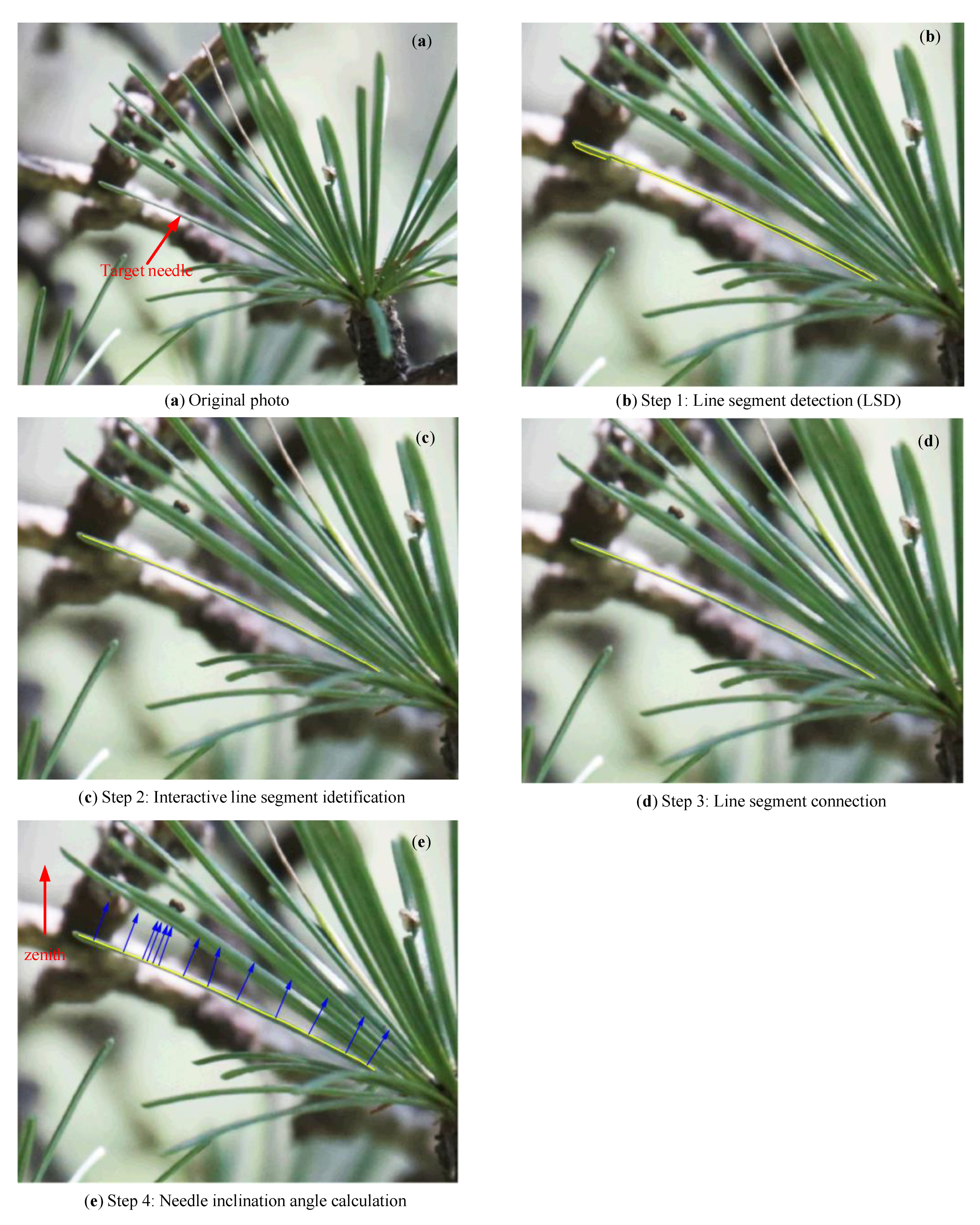
2.3.1. Needle and Shoot Inclination Angle Estimation

Collected images were further visually inspected for the presence of typical shoots with the major axis of their cylindrical brachyplast or needles with their surfaces oriented approximately perpendicular to the viewing direction of the digital camera (Figure 1) [14,28]. Therefore, for uncurved needles, the selected needles appeared as straight lines in the images. Shoot or needle samples, which were selected for SIDF or NIDF determination, were randomly selected from all available samples in the collected images. The selection was performed by two experienced operators (the two authors of this paper) to reduce the influence of operator subjectivity on the shoot or needle sample selection [14]. All samples used in this study were first selected by one of the two operators and then checked by another operator individually. Incomplete and abnormal (untypical) shoots or needles were discarded before SIDF and NIDF determination. Severely curved needles were also discarded due to the difficulty of manually obtaining stable and reliable measurements for such samples. The inclination angles of the selected shoots or needles were measured by using ACDSee Photo Manager 12 (ACD Systems International Inc., Bellevue, WA, USA) (free version) (referred as the manual method). For lightly curved needles, three inclination angle measurements were calculated for each needle sample at the middle location of three even subsections of the needle. Then, the inclination angle measurement of the curved needle sample was obtained by averaging the three inclination angle measurements.
Since the selected uncurved needle samples appeared as straight lines in the images, in order to reduce the impact of the user subjectivity of the manual method as described above on the NIDFs, a quasi-automatic method for detection of the boundary lines and further estimation of the needle inclination angles of the selected needles was developed based on a line segment detector (LSD) algorithm [35,36]. The LSD algorithm is an excellent line segment detection algorithm when compared to the traditional methods involving the combination of a canny edge detector and Hough transform, as these methods generally produce a large number of false detections [35,36,37]. For LSD, a line segment is detected as an estimate from a line support region (where pixels within that region have a similar gradient orientation value) if it passes a meaningful alignment criterion test [36,38]. The performance of the LSD in terms of detection of line segments under varying and complex field conditions has been verified previously [35,37,39,40,41]. More details of the LSD can be found in [36]. The LSD code can be publicly downloaded at http://www.ipol.im/pub/art/2012/gjmr-lsd/. Figure 2 shows a flow chart of the quasi-automatic method used to obtain the needle inclination angle measurements based on the LSD. This method includes four main steps: (1) line segment detection based on the LSD algorithm; (2) interactive line segment identification; (3) line segment connection; (4) needle inclination angle calculation. The line segments extracted using the LSD in step 1 were not perfect, since false line segments and two boundary lines were sometimes detected (Figure 2b). Since the photographs were taken at different height levels of the forest canopies and the backgrounds vary between photographs. Moreover, the boundary line shapes of the selected needles also differed. Instead of developing a totally automatic method to identify the false and redundant line segments, which could be unstable due to the varying background and boundary line shapes, an interactive identification method with the operators was used to identify the extracted effective line segments used for the needle inclination angle estimation (Figure 2c). Step 3 was used to connect the identified disconnected line segments into a whole line (Figure 2d). Then, the inclination angle of each line segment was estimated as the angle between the zenith and normal direction of each line segment (step 4) (Figure 2e). Finally, the needle inclination angle is the sum of the inclination angle of each line segment, which is achieved by multiplying its weight. The weight of each line segment was calculated by dividing the line segment length by the length of all line segments for that needle. A two-sample Kolmogorov–Smirnov (K–S) homogeneity test was adopted to evaluate whether the NIDFs of the manual and quasi-automatic methods were part of the same population [28,42].
The inclination angle measurements of the selected needles or shoots for each plot were almost evenly distributed at each height level (Table 2 and Table 3). Pisek et al. (2013) suggested that a minimum of 75 leaf inclination angle measurements is sufficient to obtain a statistically representative LIDF. Therefore, in accordance with Pisek et al. (2013), we collected at least 82 effective needle or shoot inclination angle measurements at each height level in the five plots (Table 2 and Table 3). The numbers of effective needle inclination angle measurements at each height level were larger than those of shoots (Table 2 and Table 3) because the numbers of needles were dozens of times larger than those of shoots in the canopy. Therefore, needles with their orientations perpendicular to the viewing direction of the camera were easier to be identified from the images than shoots.

2.3.2. Fitting the Needle and Shoot Inclination Angle Measurements

The SIDFs or NIDFs of each plot were derived on the basis of the obtained needle or shoot inclination angle ( θ n or θ s ) measurements. Several typical distributions, including two-parameter beta distribution, ellipsoidal distribution, and rotated-ellipsoidal distribution values, have been proposed to describe the LIDFs of vegetation canopy [43]. Among the mentioned typical functions, the two-parameter beta and ellipsoidal distributions were the two commonly used distributions adopted to fit the field leaf inclination angle measurements of vegetation canopies [1,10,14,17,30,43,44]. Since no studies have attempted to compare the performance of the beta and ellipsoidal distributions to fit the field-collected θ n or θ s measurements of coniferous forest canopies, both of the two typical distributions were used to fit the field-collected θ n or θ s measurements in this study. The probability of θ n or θ s can be described using the two-parameter beta distribution as follows [43]:
f ( t ) = 1 B ( μ , ν ) ( 1 t ) μ 1 t ν 1 ,
where t = 2 θ n / π or 2 θ s / π . The beta distribution function B ( μ , ν ) is defined as:
B ( μ , ν ) = 0 1 ( 1 x ) μ 1 x ν 1 d x = Γ ( μ ) Γ ( ν ) Γ ( μ + ν ) ,
where Γ is the gamma function, and μ and ν are the two parameters of the beta distribution function, which can be calculated as follows:
μ = ( 1 t ¯ ) ( σ 0 2 σ t 2 1 ) ,
ν = t ¯ ( σ 0 2 σ t 2 1 ) ,
where σ 0 2 is the maximum standard deviation with the expected mean t , and σ t 2 is the variance of t [43].
Similarly, the probability of θ n or θ s can also be described using the ellipsoidal distribution as follows [43,45]:
f ( θ ) = 2 χ 3 sin ( θ ) Λ ( cos ( θ ) 2 + χ 2 sin ( θ ) 2 ) 2 ,
where θ represents the needle or shoot inclination angle ( θ n or θ s ), χ is the ratio of horizontal semi-axis length to the vertical semi-axis length of an ellipsoid, and Λ is the normalized ellipse area for the projection of an ellipsoid. The ellipsoidal distribution becomes spherical distribution if χ = 1 and Λ = 2 . If χ < 1 ,
Λ = χ + sin ϵ 1 ϵ ,   ϵ = ( 1 χ 2 ) 1 / 2 ,
and if χ > 1,
Λ = χ + ln [ ( 1 + ϵ ) / ( 1 ϵ ) ] 2 ϵ χ ,   ϵ = ( 1 χ 2 ) 1 / 2 ,
The χ can be derived based on the mean value of θ n or θ s measurements ( θ ¯ ) as follows [43]:
χ = 3 + ( θ ¯ 9.65 ) 0.6061 ,
The θ ¯ estimates can be calculated using the field-collected θ n or θ s measurements as follows [43]:
θ ¯ = i = 0 90 θ j f j
where f j is the leaf area fraction for a needle or shoot angle interval centered at θ j .
All of the needle and shoot inclination angle measurements acquired in this study were fitted using two-parameter beta or ellipsoidal distribution before subsequent processing. After this, the deviation ( f D ) between the derived beta or ellipsoidal distribution and those without fitting by the two distributions ( f L D P ( θ ) ) was quantified using the modified inclination index proposed by Ross [46], which was adopted in previous studies [3,14,29]:
f D = 0 π / 2 | f ( θ ) f L D P ( θ ) | d θ   or   f D = 0 1 | f ( t ) f L D P ( t ) | d t
where f L D P ( θ ) or f L D P ( t ) is the field NIDF or SIDF, which are presented here as histograms with the bin width of 5°.
Besides the beta and ellipsoidal distributions, an additional solution except the field method used to derive the LIDFs, NIDFs, or SIDFs of vegetation canopies was designed based on the six theoretical distributions, including planophile, plagiophile, uniform, spherical, erectophile, and extremophile distributions (Figure 3). The six theoretical distributions were proposed based on the empirical evidence of the natural variation of leaf normal distributions and mathematical considerations used to describe the LIDFs values of vegetation canopies [14,47]. For spherical canopies, the relative frequency of the leaf inclination angles is the same as the relative frequency of the inclinations of the surface elements of a sphere. For uniform canopies, the relative frequency of the leaf inclination angles is the same at any angle. Planophile canopies are characterized by a predominance of horizontally oriented leaves. Plagiophile canopies are dominated by inclined leaves, erectophile canopies are dominated by vertically oriented leaves, and extremophile canopies are dominated by high frequencies of both horizontally and vertically oriented leaves [14,48] (Figure 3).

2.3.3. Needle and Shoot Projection Function Calculation

Assuming that needle azimuth angle is uniformly distributed and the needle inclination angle distribution is independent of needle size [14], then the needle projection function ( G n ( θ ) ) can be calculated as follows:
G n ( θ ) = 0 π 2 A ( θ , θ n ) f ( θ n ) d θ n ,  
A ( θ , θ n ) = { cos θ cos θ n                             | cot θ cot θ n | > 1 cos θ cos θ n [ 1 + ( 2 π ) ( tan ψ ψ ) ]               | cot θ cot θ n | 1 ,  
where θ is the view zenith and ψ = cos 1 ( cot θ cot θ n ) .
Light can penetrate through the shoots of L. principis-rupprechtii trees due to the small gaps between the needles of each shoot. Therefore, the shoot projection function ( G s ( θ ) ) cannot be derived directly from SIDF measurements by using the method described above for needles. The needle-to-shoot area ratio ( γ ) is a parameter describing the ratio between the shoot projection area and total needle area in a shoot. Therefore, a simple and applicable method for determining the G s ( θ ) of L. principis-rupprechtii forest plots based on the G n ( θ ) and γ measurements was used here as follows:
G s ( θ ) = G n ( θ ) / γ
The γ values for the five plots were obtained during the field campaign in 2017. A detailed description of the γ determination procedure can be found in [31]. We only provide a brief description here. Two to four typical shoot samples were randomly clipped from each height class (i.e., top, middle, and bottom) of the canopy in each plot. The method for γ calculation described by Chen et al. [49] was adopted in that study. The projection images of each typical shoot were taken by using a Canon 6D camera equipped with a Canon 24–70 mm lens and a flat, leveled white panel with two rules laid on its top surface [31]. Three projection images were taken for each typical shoot by rotating the shoot’s main axis at an azimuth angle of 0° and zenith angles of 0°, 45°, and 90° [31]. Then, three projection area estimates, namely A p ( 0 ° , 0 ° ) , A p ( 45 ° , 0 ° ) , and A p ( 90 ° , 0 ° ) , were derived for each typical shoot on the basis of the three projection images. Half of the total needle area of each typical shoot ( A n ) was estimated by using the volume displacement method [49]. The γ of each typical shoot was obtained on the basis of three projection area estimates and A n as follows [49]:
γ = A n A p ( 0 ° , 0 ° )     cos ( 15 ° )   +   A p ( 45 ° , 0 ° )     cos ( 45 ° )   +   A p ( 90 ° , 0 ° )     cos ( 75 ° ) cos ( 15 ° )   +   cos ( 45 ° )   +   cos ( 75 ° )
The γ of each plot was obtained by averaging the γ of all shoot samples of each plot [31].

3. Results and Discussion

3.1. Comparison of Manual and Quasi-Automatic Methods Used to Derive the Needle Inclination Angle Measurements

Obvious agreements were observed between the needle inclination angle measurements of manual and quasi-automatic methods (p > 0.92), regardless of the plot or height level (Table 4). The agreements were further verified by the small variations in mean needle inclination angles between the two methods in the five plots (<0.64° for 2017 and <0.84° for 2018) (Table 2). Both of these results indicate that the needle inclination angle measurements of manual and quasi-automatic methods in the five plots were part of the same population. Therefore, the quasi-automatic method developed in this study is effective for measuring the needle inclination angle measurements.
The total number of needle inclination angle measurements for the manual method is ten samples larger than those of the quasi-automatic method (Table 2) due to the quasi-automatic method failing for ten needle samples. Upon further examination, the reasons for the failure of the quasi-automatic method are the severe mutal shading between needles and the relatively low photograph quality, meaning that the whole needle boundary lines cannot be effectively detected using the LSD. The failure rate of the quasi-automatic method is very small (0.2%) and the mutal shading between needles can be reduced by changing the photograph acquisition position. Furthermore, the photograph quality can be improved by using a camera equipped with lenses with focal lengths larger than those used in this study, which is highly appropriate for acquiring photographs of needle samples located relatively far from the acquisition position. Therefore, the failure related to the ten needle samples using the quasi-automatic method found in this study is not a key factor that affects the effectiveness of the quasi-automatic method to be used to derive the needle inclination angle measurements. Hereinafter, only the NIDF and SIDF measurements obtained from the manual method were used due to the quasi-automatic method being inapplicable for the shoot inclination angle estimation.

3.2. Comparison of Beta and Ellipsoidal Distribution Functions for Fitting the Shoot or Needle Inclination Angle Measurements

Figure 4 and Figure 5 show that the beta distribution was outperformed the ellipsoidal distribution in fitting the shoot or needle inclination angle measurements, with smaller deviations ( f D ) in most cases. Moreover, the dominant trends of small shoot inclination angles for SIDF distributions were better described by the beta distribution compared with the ellipsoidal distribution (Figure 4). Obvious deviations were observed between the ellipsoidal and SIDF distributions of manual method at the zenith angle range of 0°–5° in the five plots (Figure 4). This finding is consistent with the conclusion made by Wang et al. [43], who concluded that the beta distribution outperformed the ellipsoidal distribution in most cases in fitting the field leaf inclination angle measurements of grasses, shrubs, and broadleaf trees across 50 plant species, even though the plant species covered by the two studies are obviously different. The same conclusion was also reported for four broadleaf tree species in the study by Wagner and Hagemeier [30]. Furthermore, the beta distribution has been adopted by several studies recently to fit field leaf inclination angle measurements of LDP [3,14,29,44]. Therefore, the beta distribution was chosen to fit the shoot and needle inclination angle measurements of LDP for further analysis in this study.

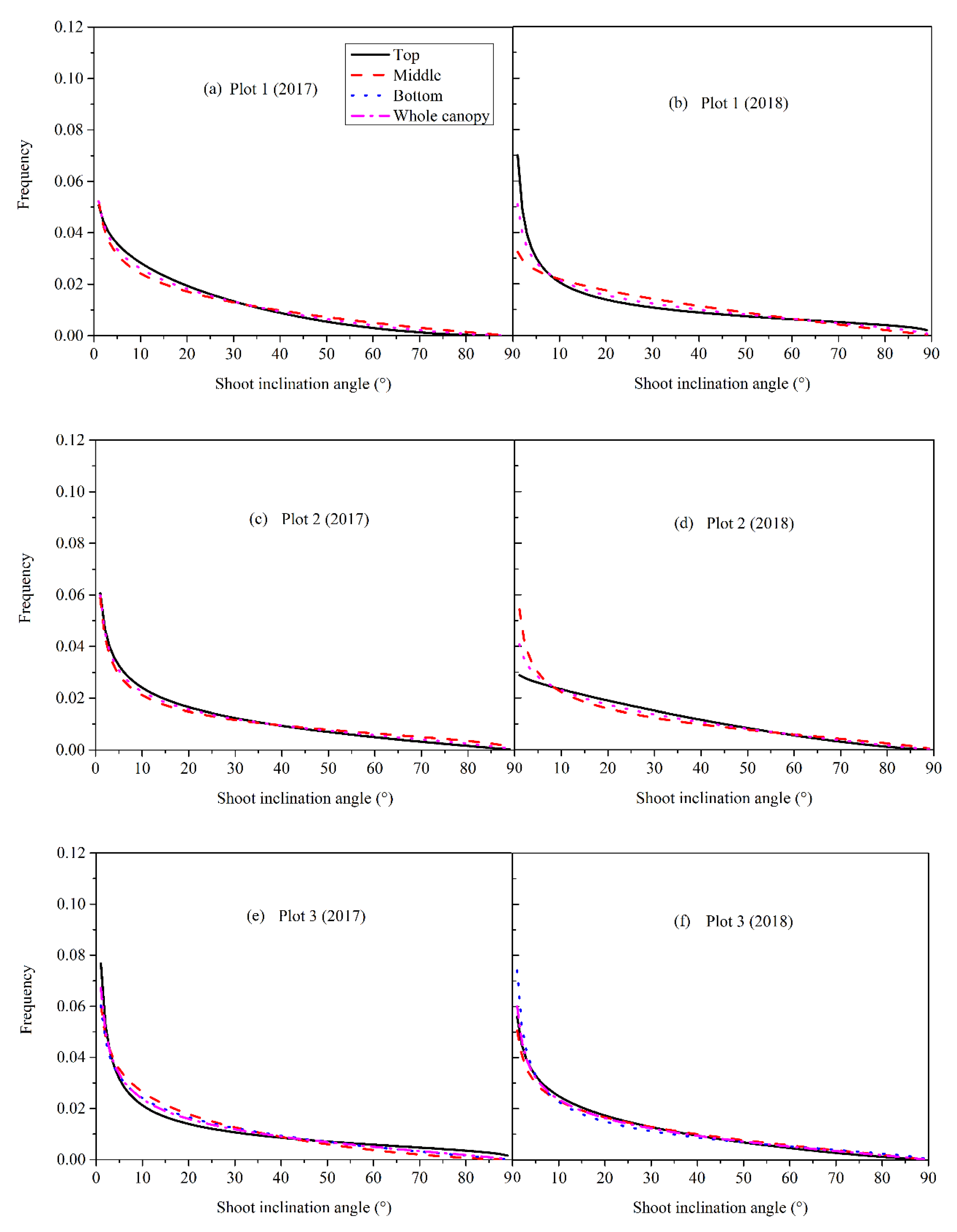
3.3. Shoot Angle Distribution

In the five plots, the SIDFs were strongly planophile (Figure 3) over the entire vertical profile throughout the 2 years (Figure 6). This phenomenon can be explained by the fact that horizontally oriented shoots were more effective than steeply inclined shoots in maximizing needle light interception from above and reducing needle light shading from neighboring needles. The reason for this is that the needles were usually distributed around the major axes of the cylindrical brachyplasts of shoots with certain angles (approximately 30°–60° in most cases, as determined through visual inspection) (Figure 1). Moreover, minor variations among the SIDFs of different height levels for the same plot were observed in all five plots (the SIDF curves at different height levels in each plot almost overlapped) (Figure 6). Minor variations were also found among the whole-canopy SIDFs of different plots for the same observation year, as well as among the whole-canopy SIDFs of different years for the same plot (Figure 6). The minor variations in SIDFs with height level and plots (whole-canopy scale) were further verified by the small variations in mean shoot inclination angles with height level and plot in the five plots (<5.37° for 2017 and <4.36° for 2018) (Table 3). Light conditions have been identified as key factors affecting the LIDFs for broadleaf forest plots [14]. The minor variations in SIDFs indicate that the SIDFs of L. principis-rupprechtii forest plots might be mainly determined by tree species and were not obviously affected by other common factors, such as light conditions, which differed within the canopies of the five plots, given that the five plots in this study exhibited contrasting forest canopy characteristics (Table 1).
On the basis of Figure 6 and Table 3, we concluded that a stable and representative SIDF measurement for L. principis-rupprechtii plots could be obtained by randomly selecting shoot samples from the canopy for a total measurement number of approximately 80–100, without considering the height level, forest plots, or light conditions. Although we did not attempt to recalculate the SIDFs of the five L. principis-rupprechtii plots by randomly choosing measurements from all available shoot inclination angle measurements of each plot, the minor variations in SIDFs with height levels, plots, and observation years (Figure 6 and Table 3) indicated that the above conclusion was valid for L. principis-rupprechtii plots.

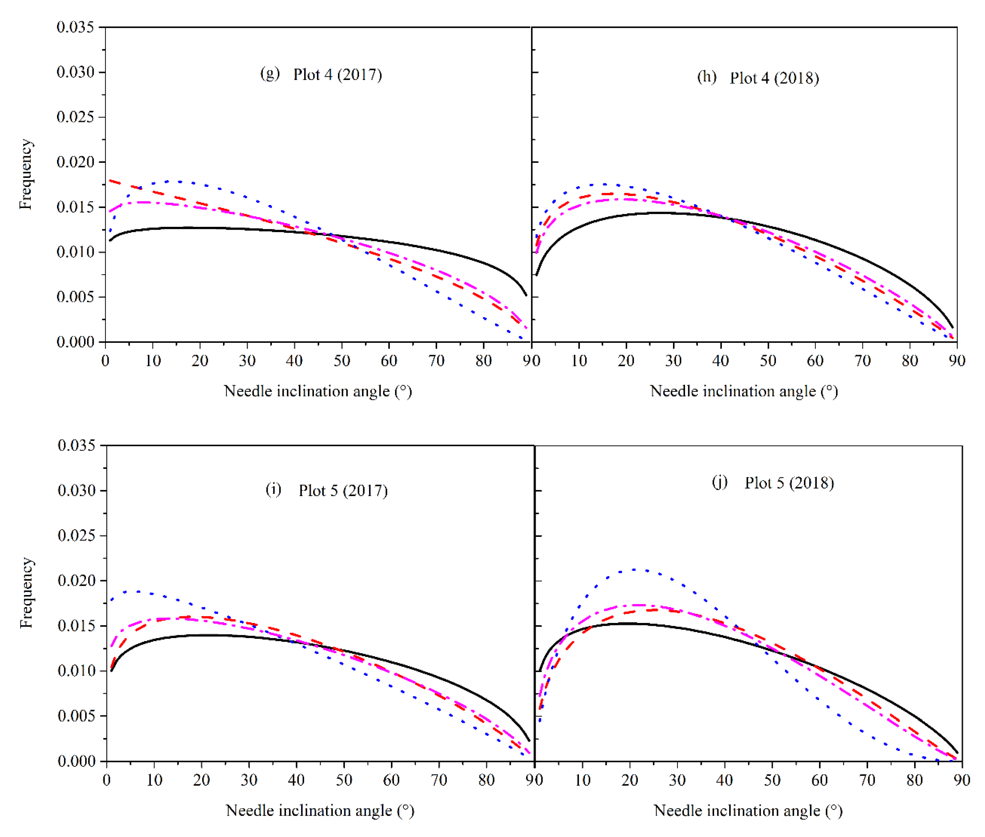
3.4. Needle Angle Distribution

The whole-canopy NIDFs for all the five plots were consistently toward the planophile throughout the 2 years (Figure 7 and Table 2). Although the tree species investigated in this study was coniferous, this finding was consistent with previous results showing that the planophile is the prevailing LIDF for broadleaf tree species in the northern hemisphere [3,14,29]. The prevalence of the planophile for broadleaf and coniferous tree species might be attributed to the greater photosynthesis in horizontal leaves than in vertical leaves for canopies with LAI values up to 6.0 in northern latitudes, according to theoretical computations [50].
Similar to the small whole-canopy SIDF variations in plots (Figure 6), no large variations were observed between the whole-canopy NIDFs for the five different plots throughout the 2 years (Figure 7). The small variations in whole-canopy NIDFs between plots were further verified by the small variations in mean needle inclination angles between plots in 2017 (<1.86°) and 2018 (<4.4°) (Table 2). Given that the five plots included very sparse (e.g., the stand densities of plots 1 and 2 ranged from 384 to 464 stems/ha) to very dense canopies (e.g., the stand density of plot 5 was 3904 stems/ha) and the LAI range of 3.04–6.69 for the five plots (Table 1), the light conditions within the canopies of the five plots were obviously different. This indicates that the variations in whole-canopy NIDFs of L. principis-rupprechtii forest plots are insensitive to light conditions. This finding is consistent with the conclusion made by Raabe et al. [14], who concluded that the variations in the LIDFs of broadleaf tree species are insensitive to light conditions if the LIDFs are planophile, because planophile function can maximize light use and improve the solar irradiance intercept efficiency of the canopy. Given the small whole-canopy NIDF variations in plots (Figure 7), a universal whole-canopy NIDF could be obtained on the basis of the NIDFs of the five plots in this study. A slight shift in zenith angles with the largest frequency was observed between the whole-canopy NIDFs for 2017 and 2018 for the same plot in the five plots (Figure 7). This shift might have been caused by the inconsistent field observation times in 2017 and 2018. Although the 2017 and 2018 field measurements were both collected at the maximum PAI period for all of the plots, the field observation times in 2017 were closer to the needle senescence period compared with those in 2018. When the needles of L. principis-rupprechtii trees approached senescence, they began to soften and the angle between the shoot main axis of the cylindrical brachyplast and needle enlarged, making the orientation of the needles close to the zenith due to the planophile SIDF. This behavior indicated that the whole-canopy NIDF values of L. principis-rupprechtii forest plots might change with seasons because the angle between the shoot main axis of the cylindrical brachyplast and needle gradually increased from the beginning of leaf emergence in late spring to the end of leaf expansion in early summer in addition to the leaf senescence period.
In most cases, small variations in NIDFs with the height levels were observed in the five plots in 2017 and 2018 (Figure 7). This trend was further verified by the relatively small differences between the mean needle inclination angles at different height levels for the same plot in the five plots (ranging from 0.02° to 9.22° in 2017 and 0.51° to 7.85° in 2018) (Table 2). Moreover, in most cases, more horizontally oriented needles were observed at the bottom level than at other two height levels in plots 3–5 and at the middle level than at the top level in plots 1–2 (Figure 7). By contrast, in most cases, more needles with oriented angles larger than 30° were observed in the top canopy compared with those at the two other height levels (Figure 7). This finding was consistent with previously reported findings for broadleaf tree species [14,51]. More needles with large inclination angles in the top canopy are helpful for reducing the amount of solar irradiance, which is usually received in excess in the top canopy especially at midday hours. The reduced solar irradiance interception at the top canopy is further helpful in increasing the amount of solar irradiance that reaches the middle and lower canopies [14,52]. By contrast, more horizontally oriented needles in the bottom canopy could improve the solar irradiance interception efficiency of the bottom canopy, because solar irradiance mainly arrives from above at directions close to the zenith [52,53]. On the other hand, the variations in the NIDFs over the entire vertical profile can increase the efficiency of the solar irradiance interception for the entire canopy [54].
Obvious differences were observed between the whole-canopy NIDFs and SIDFs from the same plot in the five plots, even though both of them showed an obvious trend of planophile distribution in most cases (Figure 6 and Figure 7). An example of this is that the mean values of the whole-canopy NIDFs were obviously larger than those of the whole-canopy SIDF for the same plot in the five plots (Table 2 and Table 3). Moreover, the zenith angles with the largest frequency for the whole-canopy NIDFs were also obviously larger than those of the whole-canopy SIDFs for the same plot in the five plots (Figure 6 and Figure 7). Therefore, we can conclude that the shoots exhibited distinct inclination angle distributions from those of needles for L. principis-rupprechtii plots.

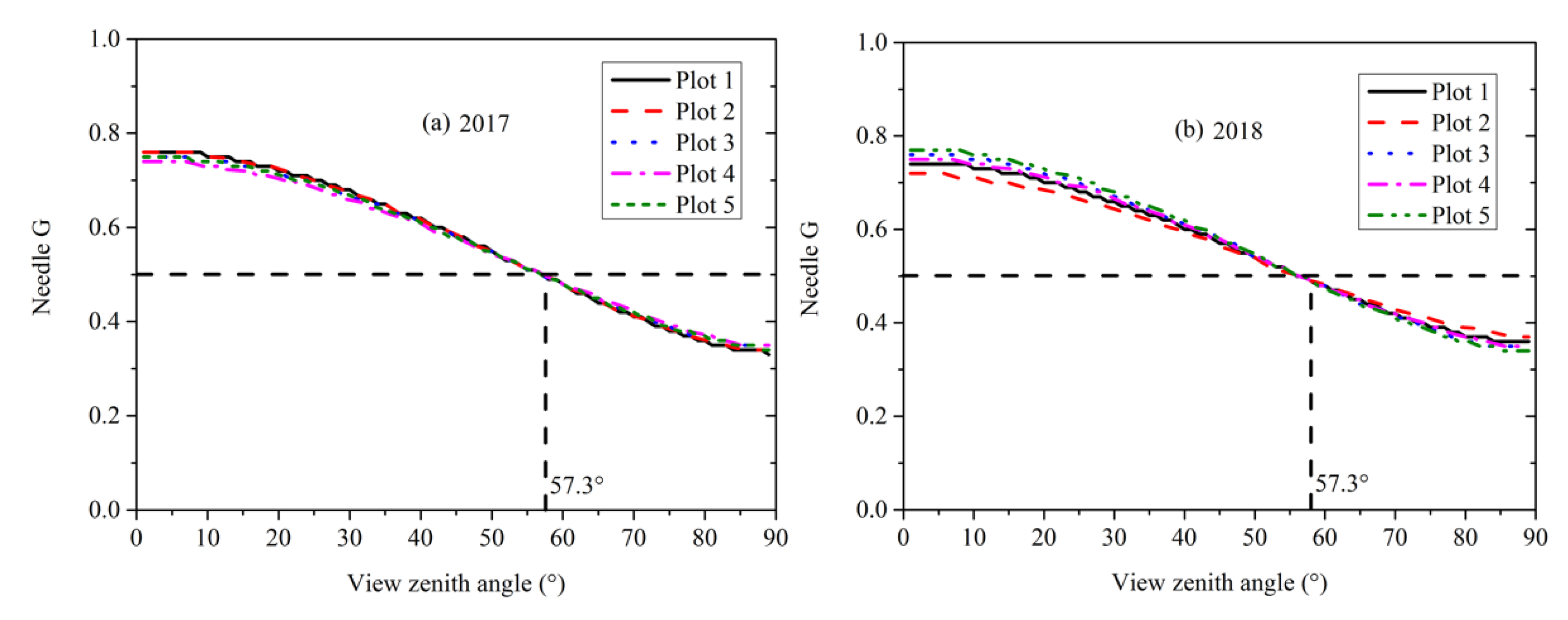
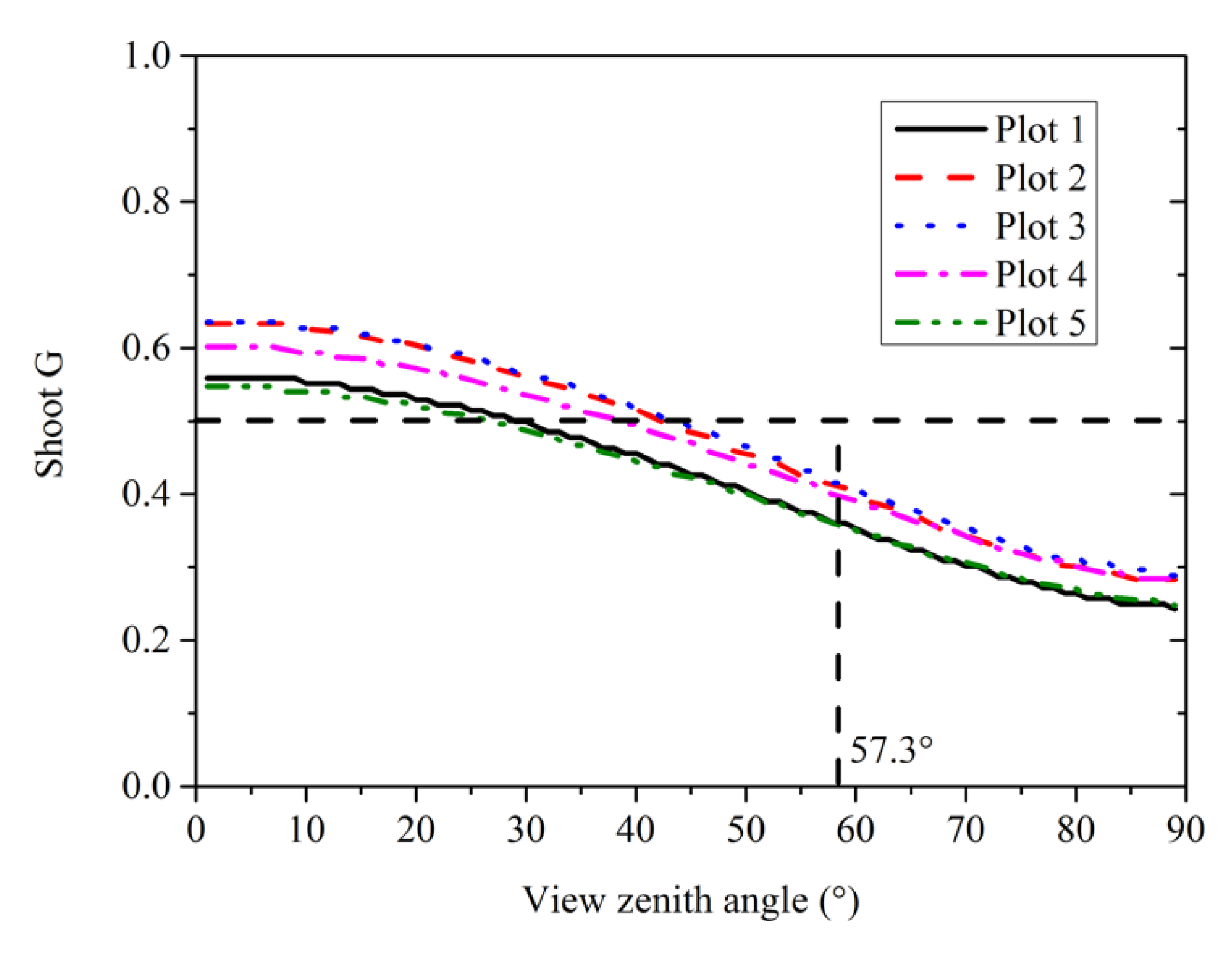
3.5. Needle and Shoot Projection Functions

The whole-canopy needle projection functions were consistently toward the planophile in all the five plots, with minor variations between plots and observation years (Figure 8). These minor variations illustrated that a representative needle projection function could be obtained for L. principis-rupprechtii plots. The needle projection functions of the five L. principis-rupprechtii plots (Figure 8) obviously deviated from the case of spherical leaf inclination distribution ( G ≡ 0.5), which has been commonly assumed for plant canopies in previous studies [2,28,29,55,56], especially at viewing directions close to the zenith (the needle G value is equal to 0.76 at 1° in plot 1) (Figure 8). Therefore, the assumption of a spherical LIDF would result in errors in the LAI and clumping index estimation for forest plots because their leaf inclination angle distributions usually deviate from the spherical case [29]. For example, Pisek et al. [29] reported that the assumption of a spherical LIDF underestimates the clumping index (28–47%) at the zenith in a birch plot. Therefore, we suggest obtaining the field leaf inclination angle distribution measurements of forest plots with tree species that have not been investigated comprehensively whenever possible. Another solution for minimizing the impact of the assumption of spherical LIDF on the LAI and clumping index estimation of forest plots without field LIDF measurements is to utilize specific characteristics of leaf or woody-component inclination angle distributions, which approximately intersect at zenith angles close to 57.3°; the values of leaf or woody-component projection coefficients at the specific zenith angle of 57.3° equal approximately 0.5 (also found in this study [Figure 8]) [55,56,57,58]. Given that the differences between the field-collected and assumed leaf or woody-component projection coefficients of forest plots at 57.3° are small, their effects on the LAI and clumping index estimation are small and acceptable [57].
Compared with the needle projection functions (Figure 8), the shoot projection functions of the five plots did not consistently approach a single typical leaf projection function and approximated the three typical leaf projection functions, namely plagiophile, uniform, and extremophile functions (Figure 9) [3,29,56]. The variations between the shoot projection functions of the five plots (Figure 9) were mainly attributed to variations in γ for the five plots due to the minor variations in needle projection functions in the plots (Figure 8). The shoot projection functions of the five plots intersected with the line of G = 0.5 at zenith angles of 27°–43° (Figure 9), which consistently deviated largely from the commonly reported intersected zenith angle of 57.3° for the leaf or woody-component projection functions of forest plots [2,29,55,56,59]. This deviation indicated that the derived shoot projection functions might contain a certain degree of estimation errors. In this study, the error in the estimated shoot projection function might originate from γ measurements, because a constant γ value was used for all viewing zenith angles in the shoot projection function estimation. However, Equation (14) shows that the γ estimates varied with zenith angles because the shoot projection areas changed with projection zenith angles. Therefore, if the method of this study is used to obtain the shoot projection function of coniferous forest plots in the future, we recommend obtaining γ estimates with zenith angles of 0°–90° and an interval of 1°, coinciding with the same zenith angle range and intervals used for needle projection functions.

4. Conclusions

The shoot and needle inclination angle distributions and projection functions of five contrasting L. principis-rupprechtii plots were obtained on the basis of the LDP method. The main conclusions of this study are as follows: (1) The quasi-automatic method developed in this study is effective and accurate enough to obtain the NIDFs. (2) The whole-canopy SIDFs and NIDFs tended to be planophile and exhibited minor variations between plots and observation years. The NIDF was slightly sensitive to light conditions given that small variations in NIDFs were observed between NIDF measurements obtained at different height levels. (3) The whole-canopy and height level needle projection functions tended to be planophile, and minor variations in needle projection functions with plots and observation years were observed. (4) The method for obtaining shoot projection functions based on needle projection functions and γ measurements used in this study tended to produce estimates with a certain degree of error, because the zenithal dependence of γ was ignored in the estimation. The performance of this method can be further evaluated by considering the variation in γ with zenith angles in the future.

Author Contributions

J.Z. proposed the concept of this study, conducted the experiment, analyzed the data, and wrote the paper. J.Z. and P.L. conducted the experiment and analyzed the data. W.H., P.Z., and Y.Z. analyzed the data. All authors have read and agreed to the published version of the manuscript.

Funding

This work was jointly funded by the National Key Research and Development Program from Ministry of Science and Technology of China (2016YFB0501501) and National Natural Science Foundation of China (Grant Nos. 41871233, 41371330, 41001203).

Institutional Review Board Statement

Not applicable.

Informed Consent Statement

Not applicable.

Data Availability Statement

The data of this work can be shared to the readers depending on the request.

Acknowledgments

We are grateful to the anonymous reviewers, whose comments much helped to improve this paper.

Conflicts of Interest

The authors declare no conflict of interest.

References

  1. Zou, X.; Mõttus, M.; Tammeorg, P.; Torres, C.L.; Takala, T.; Pisek, J.; Mäkelä, P.; Stoddard, F.L.; Pellikka, P. Photographic measurement of leaf angles in field crops. Agric. For. Meteorol. 2014, 184, 137–146. [Google Scholar] [CrossRef] [Green Version]
  2. Ross, J. The Radiation Regime and Architecture of Plant Stands; Dr. W. Junk Publ.: The Hague, The Netherlands, 1981. [Google Scholar]
  3. Chianucci, F.; Pisek, J.; Raabe, K.; Marchino, L.; Ferrara, C.; Corona, P. A dataset of leaf inclination angles for temperate and boreal broadleaf woody species. Ann. For. Sci. 2018, 75, 50. [Google Scholar] [CrossRef] [Green Version]
  4. Norman, J.M.; Campbell, G.S. Canopy structure. In Plant Physiological Ecology; Pearcy, R.W., EEhleringer, J.R., Mooney, H.A., RRundel, P.W., Eds.; Springer: Dordrecht, The Netherlands, 1989; pp. 301–325. [Google Scholar]
  5. Lang, A.R.G. Leaf orientation of a cotton plant. Agric. Meteorol. 1973, 11, 37–51. [Google Scholar] [CrossRef]
  6. Sinoquet, H.; Rivet, P. Measurement and visualization of the architecture of an adult tree based on a three-dimensional digitising device. Trees 1997, 11, 265–270. [Google Scholar] [CrossRef]
  7. Sonohat, G.; Sinoquet, H.; Kulandaivelu, V.; Combes, D.; Lescourret, F. Three-dimensional reconstruction of partially 3D-digitized peach tree canopies. Tree Physiol. 2006, 26, 337–351. [Google Scholar] [CrossRef] [Green Version]
  8. Kucharik, C.J.; Norman, J.M.; Gower, S.T. Measurements of leaf orientation, light distribution and sunlit leaf area in a boreal aspen forest. Agric. For. Meteorol. 1998, 91, 127–148. [Google Scholar] [CrossRef]
  9. Chen, J.M.; Black, T.A.; Adams, R.S. Evaluation of hemispherical photography for determining plant area index and geometry of a forest stand. Agric. For. Meteorol. 1991, 56, 129–143. [Google Scholar] [CrossRef]
  10. Wagner, S.; Hagemeier, M. Method of segmentation affects leaf inclination angle estimation in hemispherical photography. Agric. For. Meteorol. 2006, 139, 12–24. [Google Scholar] [CrossRef]
  11. Macfarlane, C.; Arndt, S.K.; Livesley, S.J.; Edgar, A.C.; White, D.A.; Adams, M.A.; Eamus, D. Estimation of leaf area index in eucalypt forest with vertical foliage, using cover and fullframe fisheye photography. For. Ecol. Manag. 2007, 242, 756–763. [Google Scholar] [CrossRef] [Green Version]
  12. Macfarlane, C.; Hoffman, M.; Eamus, D.; Kerp, N.; Higginson, S.; McMurtrie, R.; Adams, M. Estimation of leaf area index in eucalypt forest using digital photography. Agric. For. Meteorol. 2007, 143, 176–188. [Google Scholar] [CrossRef]
  13. Ryu, Y.; Sonnentag, O.; Nilson, T.; Vargas, R.; Kobayashi, H.; Wenk, R.; Baldocchi, D.D. How to quantify tree leaf area index in an open savanna ecosystem: A multi-instrument and multi-model approach. Agric. For. Meteorol. 2010, 150, 63–76. [Google Scholar] [CrossRef]
  14. Raabe, K.; Pisek, J.; Sonnentag, O.; Annuk, K. Variations of leaf inclination angle distribution with height over the growing season and light exposure for eight broadleaf tree species. Agric. For. Meteorol. 2015, 214–215, 2–11. [Google Scholar] [CrossRef]
  15. McNeil, B.E.; Pisek, J.; Lepisk, H.; Flamenco, E.A. Measuring leaf angle distribution in broadleaf canopies using UAVs. Agric. For. Meteorol. 2016, 218–219, 204–208. [Google Scholar] [CrossRef]
  16. Qi, J.; Xie, D.; Li, L.; Zhang, W.; Mu, X.; Yan, G. Estimating Leaf Angle Distribution From Smartphone Photographs. IEEE Geosci. Remote Sens. Lett. 2019, 16, 1190–1194. [Google Scholar] [CrossRef]
  17. Zheng, G.; Moskal, L.M. Leaf Orientation Retrieval From Terrestrial Laser Scanning (TLS) Data. Geosci. Remote Sens. IEEE Trans. 2012, 50, 3970–3979. [Google Scholar] [CrossRef]
  18. Hosoi, F.; Omasa, K. Factors contributing to accuracy in the estimation of the woody canopy leaf area density profile using 3D portable lidar imaging. J. Exp. Bot. 2007, 58, 3463–3473. [Google Scholar] [CrossRef] [PubMed] [Green Version]
  19. Hosoi, F.; Omasa, K. Estimating leaf inclination angle distribution of broad-leaved trees in each part of the canopies by a high-resolution portable scanning lidar. J. Agric. Meteorol. 2015, 71, 136–141. [Google Scholar] [CrossRef] [Green Version]
  20. Bailey, B.N.; Mahaffee, W.F. Rapid measurement of the three-dimensional distribution of leaf orientation and the leaf angle probability density function using terrestrial LiDAR scanning. Remote Sens. Environ. 2017, 194, 63–76. [Google Scholar] [CrossRef] [Green Version]
  21. Vicari, M.B.; Pisek, J.; Disney, M. New estimates of leaf angle distribution from terrestrial LiDAR: Comparison with measured and modelled estimates from nine broadleaf tree species. Agric. For. Meteorol. 2019, 264, 322–333. [Google Scholar] [CrossRef]
  22. Liu, J.; Skidmore, A.K.; Wang, T.; Zhu, X.; Premier, J.; Heurich, M.; Beudert, B.; Jones, S. Variation of leaf angle distribution quantified by terrestrial LiDAR in natural European beech forest. ISPRS J. Photogramm. Remote Sens. 2019, 148, 208–220. [Google Scholar] [CrossRef]
  23. Itakura, K.; Hosoi, F. Estimation of Leaf Inclination Angle in Three-Dimensional Plant Images Obtained from Lidar. Remote Sens. 2019, 11, 344. [Google Scholar] [CrossRef] [Green Version]
  24. Xu, Q.; Cao, L.; Xue, L.; Chen, B.; An, F.; Yun, T. Extraction of Leaf Biophysical Attributes Based on a Computer Graphic-based Algorithm Using Terrestrial Laser Scanning Data. Remote Sens. 2018, 11, 15. [Google Scholar] [CrossRef] [Green Version]
  25. Liu, J.; Wang, T.; Skidmore, A.K.; Jones, S.; Heurich, M.; Beudert, B.; Premier, J. Comparison of terrestrial LiDAR and digital hemispherical photography for estimating leaf angle distribution in European broadleaf beech forests. ISPRS J. Photogramm. Remote Sens. 2019, 158, 76–89. [Google Scholar] [CrossRef]
  26. Leblanc, S.G.; Chen, J.M.; Fernandes, R.; Deering, D.W.; Conley, A. Methodology comparison for canopy structure parameters extraction from digital hemispherical photography in boreal forests. Agric. For. Meteorol. 2005, 129, 187–207. [Google Scholar] [CrossRef] [Green Version]
  27. Ma, L.; Zheng, G.; Eitel, J.U.H.; Magney, T.S.; Moskal, L.M. Retrieving forest canopy extinction coefficient from terrestrial and airborne lidar. Agric. For. Meteorol. 2017, 236, 1–21. [Google Scholar] [CrossRef]
  28. Pisek, J.; Ryu, Y.; Alikas, K. Estimating leaf inclination and G-function from leveled digital camera photography in broadleaf canopies. Trees Struct. Funct. 2011, 25, 919–924. [Google Scholar] [CrossRef]
  29. Pisek, J.; Sonnentag, O.; Richardson, A.D.; Mõttus, M. Is the spherical leaf inclination angle distribution a valid assumption for temperate and boreal broadleaf tree species? Agric. For. Meteorol. 2013, 169, 186–194. [Google Scholar] [CrossRef]
  30. Utsugi, H.; Araki, M.; Kawasaki, T.; Ishizuka, M. Vertical distributions of leaf area and inclination angle, and their relationship in a 46-year-old Chamaecyparis obtusa stand. For. Ecol. Manag. 2006, 225, 104–112. [Google Scholar] [CrossRef]
  31. Zou, J.; Leng, P.; Hou, W.; Zhong, P.; Chen, L.; Mai, C.; Qian, Y.; Zuo, Y. Evaluating Two Optical Methods of Woody-to-Total Area Ratio with Destructive Measurements at Five Larix gmelinii Rupr. Forest Plots in China. Forests 2018, 9, 746. [Google Scholar] [CrossRef] [Green Version]
  32. Zou, J.; Zuo, Y.; Zhong, P.; Hou, W.; Leng, P.; Chen, B. Performance of Four Optical Methods in Estimating Leaf Area Index at Elementary Sampling Unit of Larix principis-rupprechtii Forests. Forests 2019, 11, 30. [Google Scholar] [CrossRef] [Green Version]
  33. Kimes, D.S.; Kirchner, J.A. Diurnal variations of vegetation canopy structure. Int. J. Remote Sens. 1983, 4, 257–271. [Google Scholar] [CrossRef]
  34. Zou, J.; Hou, W.; Chen, L.; Wang, Q.; Zhong, P.; Zuo, Y.; Luo, S.; Leng, P. Evaluating the impact of sampling schemes on leaf area index measurements from digital hemispherical photography in Larix gmeliniiLarix principis-rupprechtii Rupr. forest plots. For. Ecosyst. 2020, 7, 52. [Google Scholar] [CrossRef]
  35. Gioi, R.G.v.; Jakubowicz, J.; Morel, J.; Randall, G. LSD: A Fast Line Segment Detector with a False Detection Control. IEEE Trans. Pattern Anal. Mach. Intell. 2010, 32, 722–732. [Google Scholar] [CrossRef] [PubMed]
  36. Gioi, R.G.v.; Jakubowicz, J.; Morel, J.-M.; Randall, G. LSD: A Line Segment Detector. Image Process. Line 2012, 2, 35–55. [Google Scholar] [CrossRef] [Green Version]
  37. Lin, Y.; Wang, C.; Cheng, J.; Chen, B.; Jia, F.; Chen, Z.; Li, J. Line segment extraction for large scale unorganized point clouds. ISPRS J. Photogramm. Remote Sens. 2015, 102, 172–183. [Google Scholar] [CrossRef]
  38. Cho, N.; Yuille, A.; Lee, S. A Novel Linelet-Based Representation for Line Segment Detection. IEEE Trans. Pattern Anal. Mach. Intell. 2018, 40, 1195–1208. [Google Scholar] [CrossRef]
  39. Hofer, M.; Maurer, M.; Bischof, H. Efficient 3D scene abstraction using line segments. Comput. Vis. Image Underst. 2017, 157, 167–178. [Google Scholar] [CrossRef]
  40. Tang, G.; Xiao, Z.; Liu, Q.; Liu, H. A Novel Airport Detection Method via Line Segment Classification and Texture Classification. IEEE Geosci. Remote Sens. Lett. 2015, 12, 2408–2412. [Google Scholar] [CrossRef]
  41. Sun, Y.; Zhao, L.; Huang, S.; Yan, L.; Dissanayake, G. Line matching based on planar homography for stereo aerial images. ISPRS J. Photogramm. Remote Sens. 2015, 104, 1–17. [Google Scholar] [CrossRef] [Green Version]
  42. W.H. Freeman and Company. Biometry: Principles and Practice of Statistics in Biological Research, 2nd ed.; W.H. Freeman and Company: San Francisco, CA, USA, 1981. [Google Scholar]
  43. Wang, W.M.; Li, Z.L.; Su, H.B. Comparison of leaf angle distribution functions: Effects on extinction coefficient and fraction of sunlit foliage. Agric. For. Meteorol. 2007, 143, 106–122. [Google Scholar] [CrossRef]
  44. Pisek, J.; Lang, M.; Nilson, T.; Korhonen, L.; Karu, H. Comparison of methods for measuring gap size distribution and canopy nonrandomness at Järvselja RAMI (RAdiation transfer Model Intercomparison) test sites. Agric. For. Meteorol. 2011, 151, 365–377. [Google Scholar] [CrossRef]
  45. Campbell, G.S. Derivation of an angle density function for canopies with ellipsoidal leaf angle distributions. Agric. For. Meteorol. 1990, 49, 173–176. [Google Scholar] [CrossRef]
  46. Ross, J. Radiative transfer in plant communities. In Vegetation and the Atmosphere; Monteith, J.L., Ed.; Academic Press: London, UK, 1975; Volume 1, pp. 13–55. [Google Scholar]
  47. De Wit, C.T. Photosynthesis of Leaf Canopies; Wageningen University: Wageningen, The Netherlands, 1965. [Google Scholar]
  48. Lemeur, R.; Blad, B.L. A critical review of light models for estimating the shortwave radiation regime of plant canopies. Agric. Meteorol. 1974, 14, 255–286. [Google Scholar] [CrossRef]
  49. Chen, J.M.; Rich, P.M.; Gower, S.T.; Norman, J.M.; Plummer, S. Leaf area index of boreal forests: Theory, techniques and measurements. J. Geophys. Res. 1997, 102, 29429–29443. [Google Scholar] [CrossRef]
  50. Oker-Blom, P.; Kellomäki, S. Effect of angular distribution of foliage on light absorption and photosynthesis in the plant canopy: Theoretical computations. Agric. Meteorol. 1982, 26, 105–116. [Google Scholar] [CrossRef]
  51. Kull, O.; Broadmeadow, M.; Kruijt, B.; Meir, P. Light distribution and foliage structure in an oak canopy. Trees 1999, 14, 55–64. [Google Scholar] [CrossRef]
  52. Niinemets, Ü. A review of light interception in plant stands from leaf to canopy in different plant functional types and in species with varying shade tolerance. Ecol. Res. 2010, 25, 693–714. [Google Scholar] [CrossRef]
  53. King, D.A. The Functional Significance of Leaf Angle in Eucalyptus. Aust. J. Bot. 1997, 45, 619–639. [Google Scholar] [CrossRef]
  54. Cescatti, A.; Alessandro, U. Leaf to Landscape. In Photosynthetic Adaptation: Chloroplast to Landscape; Smith, W.K., Vogelmann, T.C., Critchley, C., Eds.; Springer: Berlin/Heidelberg, Germany, 2004; pp. 42–85. [Google Scholar]
  55. Weiss, M.; Baret, F.; Smith, G.J.; Jonckheere, I.; Coppin, P. Review of methods for in situ leaf area index (LAI) determination: Part II. Estimation of LAI, errors and sampling. Agric. For. Meteorol. 2004, 121, 37–53. [Google Scholar] [CrossRef]
  56. Yan, G.; Hu, R.; Luo, J.; Weiss, M.; Jiang, H.; Mu, X.; Xie, D.; Zhang, W. Review of indirect optical measurements of leaf area index: Recent advances, challenges, and perspectives. Agric. For. Meteorol. 2019, 265, 390–411. [Google Scholar] [CrossRef]
  57. Zou, J.; Zhuang, Y.; Chianucci, F.; Mai, C.; Lin, W.; Leng, P.; Luo, S.; Yan, B. Comparison of Seven Inversion Models for Estimating Plant and Woody Area Indices of Leaf-on and Leaf-off Forest Canopy Using Explicit 3D Forest Scenes. Remote Sens. 2018, 10, 1297. [Google Scholar] [CrossRef] [Green Version]
  58. Woodgate, W. In-Situ Leaf Area Index Estimate Uncertainty in Forests: Supporting Earth Observation Product Calibration and Validation. Ph.D. Thesis, RMIT University, Melbourne, Australia, 2015. [Google Scholar]
  59. Woodgate, W.; Disney, M.; Armston, J.D.; Jones, S.D.; Suarez, L.; Hill, M.J.; Wilkes, P.; Soto-Berelov, M.; Haywood, A.; Mellor, A. An improved theoretical model of canopy gap probability for Leaf Area Index estimation in woody ecosystems. For. Ecol. Manag. 2015, 358, 303–320. [Google Scholar] [CrossRef]
Figure 1. Example of the determination of the needle or shoot inclination angles based on the leveled digital photography method. Here, Z denotes the zenith, N n denotes the needle surface normal, and N s denotes the major axis of the cylindrical shoot brachyplast; θ n and θ s are the needle and shoot inclination angles, respectively.
Forests 12 00030 g001
Figure 2. The flow chart of the quasi-automatic method used to measure the needle inclination angle based on the line segment detector (LSD) algorithm and photographs acquired by the leveled digital photography method. The target needle (a) is the same as the target in Figure 1. The blue lines and arrows (e) denote the normal directions of the line segments detected by LSD.
Forests 12 00030 g002
Figure 3. Beta distributions for the six theoretical leaf inclination angle distributions proposed by de Wit [47].
Forests 12 00030 g003
Figure 4. A comparison of the beta and ellipsoidal distribution functions used to fit the whole-canopy shoot inclination angle measurements, which were manually obtained from the leveled digital photography (LDP) method in the five plots. The shoot inclination angle distributions of the LDP method are presented as histograms with a bin width of 5°. Only the whole-canopy shoot inclination angle measurements from 2018 are shown here, as the shoot inclination angle measurements at the three height levels (i.e., bottom, middle, and top) and those from 2017 showed similar behavior.
Forests 12 00030 g004aForests 12 00030 g004b
Figure 5. A comparison of the beta and ellipsoidal distribution functions used to fit the whole-canopy needle inclination angle measurements in the five plots. Only the whole-canopy needle inclination angle measurements from 2018 are shown here, as the needle inclination angle measurements at the three height levels (i.e., bottom, middle and top) and those from 2017 showed similar behavior.
Forests 12 00030 g005aForests 12 00030 g005b
Figure 6. Vertical and annual variations in shoot inclination angle distribution in the five plots in 2017 and 2018.
Forests 12 00030 g006aForests 12 00030 g006b
Figure 7. Vertical and annual variations in needle inclination angle distributions in the five plots in 2017 and 2018.
Forests 12 00030 g007aForests 12 00030 g007b
Figure 8. Whole-canopy needle projection function against viewed zenith angles in the five plots in 2017 (a) and 2018 (b).
Forests 12 00030 g008
Figure 9. Derived whole-canopy shoot projection function against viewed zenith angles in the five plots in 2017.
Forests 12 00030 g009
Table 1. Characteristics of Larix principis-rupprechtii plots [31].
Plot 1Plot 2Plot 3Plot 4Plot 5
Longitude and latitudeN 42°24′43″,
E 117°19′4″
N 42°24′2″,
E 117°18′40″
N 42°18′2″,
E 117°18′9″
N 42°25′22″,
E 117°19′32″
N 42°17′42″,
E 117°16′53″
Mean tree height (m) *19.420.412.613.38.7
Average diameter at breast height (cm)26.627.212.714.19.2
Stand density (stems/ha)464384232017603904
Tree age (~years)5455212213
Needle-to-shoot area ratio ( γ ) **1.361.201.181.231.37
Litter collection LAI ***4.653.584.963.046.69
Tree speciesLarix principis-rupprechtii
* The height of each tree in each plot was estimated based the point cloud dataset collected using the terrestrial laser scanner in the 2017 leaf area index (LAI) measurement campaign [31]. The height of each tree was calculated as the vertical distance between the highest point of the tree and the lowest point of the stem located close to the ground [31]. ** The needle-to-shoot area ratio ( γ ) of each plot was estimated by averaging the γ of typical shoot samples harvested from the three height levels of forest canopies (i.e., top, middle, and bottom). Details of γ estimation can be found in Section 2.3.3. *** The litter collection LAI of the five plots was obtained by using the litter collection measurements acquired in the 2017 LAI measurement campaign [32].
Table 2. Statistical characteristics (i.e., number of measurements (count), mean needle inclination angle (mean), and standard deviation (SD)) of the needle inclination angle distribution function (NIDF) measurements, which were derived using the manual and quasi-automatic estimation methods, respectively, in the five plots. The quasi-automatic method failed for ten needle samples, the results of which were not included for the quasi-automatic method measurements.
Plot NameHeight LevelManualQuasi-Automatic
2017201820172018
CountMeanSDCountMeanSDCountMeanSDCountMeanSD
Plot 1Top19234.5222.1814640.9622.019235.0422.3014641.7521.67
Middle18934.522.4415833.1120.8218934.7022.3215833.4320.85
Bottom\ *\\\\\\\\\\\
All38134.5122.2830436.8821.7238134.8722.2830437.4321.62
Plot 2Top14139.1922.8725938.2722.9914139.5922.4925939.1123.07
Middle13629.9720.7225039.8822.0113630.0220.6325040.6322.13
Bottom\\\\\\\\\\\\
All27734.6622.2850939.0622.5127734.8922.0850939.8622.60
Plot 3Top1343922.9122736.2722.013439.0522.8122736.9222.08
Middle13531.9921.5222335.1421.6413532.3720.9822335.4721.64
Bottom12435.7922.7222234.6320.5912436.1122.5122234.8220.31
All39335.5822.5167235.3621.4039335.6822.4567235.7521.35
Plot 4Top17041.5924.7410839.722.7517042.1924.6610839.6222.83
Middle17134.5923.0910634.8821.5717034.6523.1210634.7020.87
Bottom16032.7120.839833.2420.9615733.0120.659833.6020.96
All50136.3723.2631236.0421.949736.7123.2331236.0521.69
Plot 5Top22239.3523.4418537.022.3822239.9923.2918537.6222.24
Middle22235.7121.8817336.22520.6222135.8821.5417336.8120.32
Bottom21231.8921.5618530.8517.5121232.0821.3218531.6417.48
All65635.7122.4954334.6620.4165536.0422.2854335.3220.24
* Not applicable.
Table 3. Statistical characteristics (i.e., number of measurements (count), mean shoot inclination angle (mean), and standard deviation (SD)) of the shoot inclination angle distribution function (SIDF) measurements, which were derived using the manual estimation method in the five plots.
Plot NameHeight Level20172018Plot NameHeight Level20172018
CountMeanSDCountMeanSDCountMeanSDCountMeanSD
Plot 1Top9019.6816.918324.7324.2Plot 2Top9222.2720.479625.9119.46
Middle8623.0620.188527.3121Middle8825.6723.49024.7621.97
Bottom\*\\\\\Bottom\\\\\\
All17621.3318.616826.0422.6All18023.9321.9618625.3520.67
Plot 3Top9423.123.589221.9319.6Plot 4Top9024.2822.128323.8119.77
Middle9420.1418.379724.3221.08Middle9425.3722.088421.419.41
Bottom9022.2620.439721.9621.94Bottom8921.3419.818220.4619.56
All27821.8320.8728622.7520.87All27323.721.3724921.919.55
Plot 5Top13825.6723.178421.322.88
Middle13420.320.538622.3522.25
Bottom13820.8219.789221.4121.44
All41022.2921.326221.6822.09
* Not applicable.
Table 4. The results of the Kolmogorov–Smirnov test comparing the manual and quasi-automatic measurements of needle inclination angle measurements in the five plots. D and P are the maximum difference between the cumulative distributions (D) and the corresponding level of probability (P).
Plot NameHeight Level20172018Plot NameHeight Level20172018
DPDPDPDP
Plot 1Top0.031.00.050.99Plot 2Top0.041.00.030.99
Middle0.031.00.040.99Middle0.041.00.040.95
Bottom\*\\\Bottom\\\\
All0.021.00.030.99All0.031.00.030.97
Plot 3Top0.060.940.041.0Plot 4Top0.041.00.041.0
Middle0.050.980.031.0Middle0.031.00.041.0
Bottom0.041.00.031.0Bottom0.050.970.041.0
All0.031.00.020.99All0.021.00.031.0
Plot 5Top0.031.00.031.0
Middle0.040.980.041.0
Bottom0.040.990.050.92
All0.021.00.030.93
* Not applicable.
Publisher’s Note: MDPI stays neutral with regard to jurisdictional claims in published maps and institutional affiliations.

