Analysis of Taper Functions for Larix olgensis Using Mixed Models and TLS

Abstract

Terrestrial laser scanning (TLS) plays a significant role in forest resource investigation, forest parameter inversion and tree 3D model reconstruction. TLS can accurately, quickly and nondestructively obtain 3D structural information of standing trees. TLS data, rather than felled wood data, were used to construct a mixed model of the taper function based on the tree effect, and the TLS data extraction and model prediction effects were evaluated to derive the stem diameter and volume. TLS was applied to a total of 580 trees in the nine larch (Larix olgensis) forest plots, and another 30 were applied to a stem analysis in Mengjiagang. First, the diameter accuracies at different heights of the stem analysis were analyzed from the TLS data. Then, the stem analysis data and TLS data were used to establish the stem taper function and select the optimal basic model to determine a mixed model based on the tree effect. Six basic models were fitted, and the taper equation was comprehensively evaluated by various statistical metrics. Finally, the optimal mixed model of the plot was used to derive stem diameters and trunk volumes. The stem diameter accuracy obtained by TLS was >98%. The taper function fitting results of these data were approximately the same, and the optimal basic model was Kozak (2002)-II. For the tree effect, a₆ and a₉ were used as the mixed parameters, the mixed model showed the best fit, and the accuracy of the optimal mixed model reached 99.72%.The mixed model accuracy for predicting the tree diameter was between 74.22% and 97.68%, with a volume estimation accuracy of 96.38%. Relative height 70 (RH70) was the optimum height for extraction, and the fitting accuracy of the mixed model was higher than that of the basic model.

1. Introduction

The taper equation is a mathematical function that studies the diameter of any part of the stem and the corresponding tree height (TH), total TH, and diameter at breast height. The taper function has a wide range of applications in tree stem volume estimation, 3D space model reconstruction, yield estimation, forest planning, and timber production simulation and optimization [1,2]. The taper equation can be used to estimate the diameter at any height on the stem, the height at any diameter, the total stem volume, and the merchantable volume of different specifications [3,4,5]. A simplified Kozak variable-exponential taper function can improve the predictive ability of the model by adding an auxiliary diameter through the mixed effect method [6]. The fixed effect model is simpler than the mixed effect model. However, the mixed model eliminates the error correlation and heterogeneity of hierarchical data, to improve the prediction accuracy of the model and explain the source of random errors [7]. Doyog N D’s study of compatible “Max and Burkhart (1976)” showed that the estimated value of the bottom diameter of the trunk is higher than the true value, while the middle and upper diameters are underestimated; the overall height and volume of the stem at a given diameter are overestimated [8]. A compatible system composed of the taper equation, total volume equation and volume sales equation was used for the modeling, and the fitting accuracy of the optimal model reached 98% [9]. Not only biological factors but also abiotic factors affect the trend of the stem curve, such as climate, soil, water, and altitude [5,10]. In addition, the relationship between the crown width (CW), stand density, thinning intensity, site quality and the taper equation has been explored [11]. Jiang et al. [12] adopted a nonlinear mixed model to fit the stem taper equation of Larix gmelinii with crown characteristics. This model shows that the stem taper is related to the crown ratio, and a large crown ratio had a poor shape quality. Cai Jian et al. [13] proposed that the tree shape of moderate thinning (35.7% of the plants removed) was relatively full.

Lidar is an active remote sensing technique that actively measures the target and detect its position, shape, height and other parameters by emitting and receiving laser pulses. Terrestrial laser scanning (TLS) emerged in the 1990s. TLS are instruments that enable the nondestructive, rapid and precise digitization of physical scenes into three-dimensional (3D) point clouds [14]. A modern TLS system can densely scan underneath the canopy surroundings within a few hundred meters with high accuracy [15]. Compared to traditional field inventories, TLS can obtain relatively complete 3D coordinate information, which can be reconstructed in the form of point clouds, to truly restore the overall structure and morphological characteristics of the located objects [16]. The point cloud data obtained by TLS are dense and accurate and have the potential for automatic processing. Moreover, the resolution of the TLS forest canopy is high and is not destructive to the forest. Liang et al. [17] reported that with field measured stem from diameters as reference, an evaluation of extraction accuracy shows a mean RMSE of 1.13 cm per tree, as low as manual extraction from TLS. The 2D Hough transform and fitting circle are commonly used in forestry to identify single trees and obtain their positions and diameters at breast height (DBHs) [18]. Some researchers have proposed an octree-based ground point filtering algorithm for woodland scenes, which has enabled automatic ground point high-accuracy filtering. These scholars also proposed an algorithm for identifying trees according to the projection density of voxels, which improves the efficiency and accuracy of trunk recognition [19]. Bauwens et al. used a hand-held laser scanner consisting of a TLS scanner and additional sensors, which can be referred to as a kinematic TLS system [20]. Walking with it through the forest produced point clouds from which positions and other single tree properties could be derived. Currently, the terrestrial LiDAR technology has been used for tree crown geometry reconstruction, biomass estimation, forest parameter inversion, single tree factor extraction, and leaf area simulation. The results show that the TLS data have a higher accuracy, better simulation effect, and stronger estimation ability, with great advantages for improving the efficiency of forestry investigations.

TLS can yield 3D information of standing trees accurately, quickly and non-destructively, which greatly facilitates the potential for forest sustainability research. Previous studies showed that the DBH and TH extracted by TLS have achieved high accuracy, but there are few reports on the extraction effect of the upper stem diameter. Xi et al. reported that the treetops are heavily shaded by leaves and branches at heights above 10 m [21]. The loss of stem points in upper stems above 10 m was also reported by Henning et al. [16]. Yang et al. extracted the diameter to a height of 6 m [22]. TLS measurement still has problems with regard to data accuracy and effect verification in large-scale information acquisition [23]. To test the extraction accuracy of the entire stem, the taper equation was established using the extracted diameter to provide a new data acquisition method for estimating growing stock, as well as to enable TLS to play a greater role in forestry.

2. Materials and Methods

2.1. Data Source and Processing

In October 2019, nine larch fixed sample plots were selected in the Mengjiagang Forest Farm of Jiamusi city, Heilongjiang Province according to different site qualities, densities, ages and thinning intensities. The DBH, height, CW and relative coordinates of each tree were measured. The DBH of each plot was divided into five grades according to the method of equal cross-sectional area sample trees, and the average DBH of each grade was calculated. Six plots (there were a total of nine plots, but stem analysis was only conducted on six plots due to the weather.) were selected, and five sample trees of different sizes were chosen near the sample plots according to the average DBH of each grade for stem analysis. We collected a total of 30 trees for stem analysis. The DBH, TH, CW, and height of the tree’s crown base (HCB) based on the stem analysis were measured. The relative height according to the total tree height was calculated, and the diameter of each relative height was measured, including 0 m, RH2, RH4, RH6, RH8, RH10, RH20, RH25, RH30, RH40, RH50, RH60, RH70, RH75, RH80 and RH90.

TLS data were collected by a Trimble TX8 narrow infrared laser beam before stem analysis. Five stations were scanned for each plot, three stations were scanned for each stem analysis, and the scanning time of each station was 3 min. After data preprocessing, a total of 580 larch trees were obtained from 9 plots, and 7887 diameters at different heights were extracted; a total of 451 diameters were extracted from 30 trees for stem analysis. Seventy-five percent of the sample trees were used for model parameterization, and the remainder (25%) were used to evaluate model performance. The parameters of Trimble TX8 are listed in

Table 1. Main technical parameters of the Trimble TX8 system.

Device Type	Trimble TX8
Measurement accuracy	<2 mm
Field-of-view	360° Horizontal × 317° Vertical
Laser beam divergence	80 µrad
Mirror rotating speed	60 rps
Point spacing at 30 m	11.3 m
Number of points	138 million points
Range	120 m
Laser wavelength	1500 nm
Minimum range	0.6 m
Measurement rate	1 MHz
Resolution	0.1 mm
Scan Rate	1,000,000 points/second

. A summary of the stem analysis data is provided in

Table 2. Basic characteristics of the selected tree variables.

	DBH (cm)	TH (m)	HCB (m)	CW (m)	Age (Years)
Max	31.0	26.0	17.5	3.80	51
Min	9.0	13.2	3.3	1.54	22
Mean	18.27	18.73	10.25	1.71	1.64
Standard Deviation	5.85	3.72	4.15	0.41	0.56

.

2.2. Processing Point Cloud Data

The original scanned data were in TZF format. Trimble RealWorks11.1 and LiDAR360 software were used for registration, denoising, 0.01 m minimum point spacing for subsampling, classification of ground points with an improved progressive TIN densification filtering algorithm, establishment of the digital elevation model, normalization by ground class, point cloud segmentation, tree identity matching and other processing. The diameters at different heights were fitted by the least squares method. To reduce the influence of the tree height on the extraction accuracy, the absolute height was replaced by the relative height. The position of stem diameter extraction is shown in Figure 1. When extracting the diameter, the slice thickness was 10 cm. For example, assuming that the diameter at 1.3 m was extracted, point clouds with heights from 1.25–1.35 m were selected for the fitting circle.

In this study, the stem analysis data at each relative height of 30 felled trees were selected for verification, which also provided a basis for constructing the taper equation. The analyzed diameter of 30 trees was taken as the reference value, and the corresponding TLS data were taken as the predicted value. The extraction effect was evaluated by the coefficient of determination (R²), root mean square error (RMSE), absolute error (bias) and extraction accuracy (P%).

2.3. Basic Taper Function

Referring to the latest edition of “Forest Mensuration” (Fourth Edition) [24] and related documents worldwide, six different commonly used types of taper equations were used in this study as candidate models. The relative height values at the lower and upper inflection points of the segmented taper equation were set to RH9 and RH77, respectively [25]. Among the 30 trees in the stem analysis, 75% (23 trees) for model fitting and the remaining 25% (7 trees) for evaluation. TLS data are the same.

(1)

Simple taper equation:

Kozak (1969)-II [26]:

$$d^2/D^2=a_1\left(1-2q+q^2\right)$$

(1)

Kozak (1969) [26]:

$$d^2/D^2=a_1+a_2\left(h/H\right)+a_3{\left(h/H\right)}^2$$

(2)

Schumacher(1973) [24]:

$$d=a_1{D}^{a_2}{\left(H-h\right)}^{a_3}/H^{a_4}$$

(3)

(2)

Segmented taper equation:

Max and Burkhart (1976) [27]:

$$\begin{gathered} d^2=D^2\left[a_1\left(q-1\right)+a_2\left(q^2-1\right)+a_3{\left(RH9-q\right)}^2{I}_1+a_4{\left(RH77-q\right)}^2{I}_2\right] \\ {I}_1=1, if q\le RH9;0 otherwise \\ {I}_2=1, if q\le RH77;0 otherwise \end{gathered}$$

(4)

(3)

Variable-exponential taper equation:

Weisheng Zeng, Zhiyun Liao (1997) [28]:

$$\begin{gathered} d/D={\left(\frac{H-h}{H-1.3}\right)}^K \\ K=a_1+a_2{\left(h/H\right)}^{1/4}+a_3{\left(h/H\right)}^{1/2}+a_4\left(D/H\right) \end{gathered}$$

(5)

Kozak (2002)-II [4]:

$$\begin{gathered} d=a_1{D}^{a_2}{H}^{a_3}{\left(\frac{1-q^{1/3}}{1-t^{1/3}}\right)}^X \\ X=a_4{q}^4+a_5\left(1/e^{D/H}\right)+a_6{\left(\frac{1-q^{1/3}}{1-t^{1/3}}\right)}^{0.1}+a_7\left(1/D\right)+a_8{H}^{1-q^{1/3}}+a_9\left(\frac{1-q^{1/3}}{1-t^{1/3}}\right) \end{gathered}$$

(6)

where $d$ is the stem diameter at a height of $h$; $D$ is the diameter at breast height; $H$ is the total tree height; $h$ is the measuring point height; $a_1, a_2,a_3,\cdots ,a_9$ are the parameters of the model; $q=h/H$; and $t=1.3/H$.

2.4. Mixed Effects Models

Because the main purpose of our study was to provide the best taper model to predict the upper stem diameter for point cloud data, the fixed-effects modelling approach guided the model selection procedure. The stem diameter data have a hierarchical structure (several diameter measurements within a single sample tree) and great spatial variability. The taper equation established by the trees in the sample plots can better represent the trends in the stem curve of the forest stand and can also more accurately predict the upper diameter of the trunk and estimate the volume. Once the best model was selected, a nonlinear mixed model with the tree effect was fitted and compared with the fixed-effects model. The mixed model expression is as follows:

$$\{\begin{array}{c}{Y}_{ij}=f\left({\varnothing }_{ij}, x_{ij}\right)+{\epsilon }_{ij} \\ \left(i=1, \cdots , m,j=1,\cdots ,n_i \right)\\ {\varnothing }_{ij}=A_{ij}\beta +B_{ij}{b}_i\\ {\epsilon }_{ij}~N\left(0,{\sigma }^2{R}_i\right),b_i~N\left(0,D\right)\end{array}$$

(7)

where $Y_{ij}$ is the dependent variable of the $j$th observation of the $i$th tree, which refers to the diameter at the relative height in this paper; $m$ is the number of samples; $n_i$ is the number of observations of the $i$th tree; $x_{ij}$ is the relative height; $\beta$ is a $\left(p\times 1\right)$ dimensional vector of the fixed parameters; $B_{ij}$ is a $\left(q\times 1\right)$ random effects parameter vector; $A_{ij}$ and $B_{ij}$ are the corresponding design matrices; $R_i$ is a variance-covariance matrix for the error terms; ${\epsilon }_{ij}$ is an n-dimensional vector of the residuals; and ${\sigma }^2$ is the variance value.

The following three steps are used to construct the mixed effect model [29]:

(1)

Determine random parameters. Fit the taper models of different random parameter combinations and compare the fit statistics. Too many parameters may lead to the overparameterization or nonconvergence of the model. Therefore, this study only selects a combination of 1–2 random parameters for fitting and compares the Akaike information criterion (AIC), Bayesian information criterion (BIC) and log-likelihood values of the model fitting. The results show that models with a smaller AIC and BIC generally have a larger logarithmic likelihood value and better fitting quality.

(2)

Determine the variance-covariance structure within-trees (R). The data of this study has a hierarchical structure among trees, therefore, we needed to solve the problem of the correlation and heteroscedasticity of intra-tree errors. To compensate for the effects of autocorrelation, this study used the first-order autoregressive structure AR (1). This study utilized the work of Davidian (1995), which is common in forestry research, to calculate [30]:

$$R_i={\sigma }^2{G}_i^{0.5}{\Gamma }_i{G}_i^{0.5}$$

(8)

where ${\sigma }^2$ refers to the error variance value of the model; ${\Gamma }_i$ is the time series correlation structure, i.e., the error correlation structure within the tree; and $G_i$ is the diagonal matrix of the variance heterogeneity.

(3)

Determine the structure of the inter-tree variance-covariance (D). The structure of inter-tree variance-covariance reflects the changes among groups. Taking the Generalized positive—definite matrices commonly used in forestry as an example, the variance-covariance structures of 2 random parameters were selected:

$$D=\left[\begin{array}{cc}{\sigma }_u^2& {\sigma }_{uv}\\ {\sigma }_{uv}& {\sigma }_v^2\end{array}\right]$$

(9)

where ${\sigma }_u^2$ is the variance of the random parameter u, ${\sigma }_v^2$ is the variance of the random parameter v, and ${\sigma }_{uv}$ is the covariance of random parameters u and v.

2.5. Evaluation and Test Models

This study uses independent data that are not involved in modeling for testing. The test of the fixed effects parameter in the mixed effects model is equivalent to the traditional regression analysis test, and the random effect component requires secondary sampling to calculate the random parameter value. Five samples were randomly selected from each tree, and the method of Vonesh was used to calculate the random parameter values [31].

$${\widehat{b}}_i\approx \widehat{D}{\widehat{Z}}_i^T{\left({\widehat{Z}}_i\widehat{D}{\widehat{Z}}_i^T+{\widehat{R}}_i\right)}^{-1}{\widehat{e}}_i$$

(10)

where $\widehat{D}$ is the variance-covariance matrix of the random effect parameters, ${\widehat{R}}_i$ is the variance-covariance structure in the sample tree, ${\widehat{Z}}_i$ is the design matrix, and ${\widehat{e}}_i$ is the actual value minus the predicted value calculated with fixed effect parameters.

2.6. Application of the Model

2.6.1. Prediction of the Stem Diameter

The taper function can be used to estimate the diameter of any height on the tree. The mixed model was established using 580 trees from 9 plots. It is highly representative and can simulate the stem curve well. It was used in this study to derive the diameter of the upper stem that cannot be obtained by TLS. The prediction of the upper diameter, which was obtained with the mixed model, not only solves the problem of missing point cloud data but also accurately estimates the volume.

2.6.2. Estimated Volume

The ultimate purpose of constructing the taper equation is to calculate the volume. This study adopted the following three types of methods to calculate the volume of 30 trees: Method 1, the optimal taper model with tree effects was integrated numerically to compute the volume; Method 2, the extracted diameters at different relative heights were directly used to calculate the volume with the mid-area sectional measurement method (the diameter that could not be extracted from the upper stem was calculated according to the predicted value by the taper equation); and Method 3, the measured value from the stem analysis at each meter was used to calculate the volume. The measured volume (Method 3) was taken as the reference value and was compared with those of the other two methods to determine their prediction accuracies.

3. Results

3.1. Summary of TLS Extraction Data

The recognition performance of the point cloud data between the ground and the bottom of the tree is limited when establishing the digital elevation model; thus, the difference in the measured diameter of 0 m is also relatively large(to be consistent with the stem analysis, we extracted the point cloud value at 0.1 m as 0 m). Therefore, the extracted diameter at 0 m was compared with the actual measurement. The DBH, TH, HCB, CW and diameters of different positions extracted from 30 trees were analyzed.

Table 3. Summary of the point cloud-extracted data.

	n	Bias/m	RMSE/m	R2	P/%
TH (m)	30	0.1157	0.1686	0.9979	99.3578
HCB (m)	30	0.5594	1.0305	0.9406	94.5960
CW (m)	30	0.5333	0.7267	0.1732	84.7210
Diameter Extraction Position	n	Bias/cm	RMSE/cm	R2	P/%
DBH	30	0.3132	0.3726	0.9958	98.1829
0 m	30	1.3277	1.5863	0.9652	93.9117
RH2	30	0.3827	0.4685	0.9942	97.8472
RH4	30	0.3720	0.4490	0.9937	97.8882
RH6	30	0.2830	0.3419	0.9961	98.3065
RH8	30	0.2683	0.3258	0.9963	98.3216
RH10	30	0.2530	0.3145	0.9965	98.4318
RH20	30	0.3807	0.4652	0.9916	97.6410
RH25	30	0.3417	0.4588	0.9910	97.9358
RH30	30	0.3387	0.4426	0.9907	97.7912
RH40	30	0.3313	0.4069	0.9909	97.6145
RH50	30	0.3840	0.4871	0.9834	96.7759
RH60	30	0.4610	0.5707	0.9737	95.6473
RH70	30	0.4190	0.5931	0.9640	94.7987
RH75	30	0.6140	0.8258	0.9228	90.7241
RH80	24	0.4963	0.6441	0.9237	91.7222
RH90	7	0.4686	0.5449	0.7823	85.5083

shows a summary of the point cloud-extracted data. When the tree height was between RH75 and RH90, the diameter of some point clouds could not be extracted due to the occlusion caused by branches and leaves.

Most of the R² values extracted from the diameters at 15 different relative heights were more than 0.92. The extraction results of the DBH and tree height are good, with accuracies of 98.18% and 99.36%, respectively. The accuracy of the HCB was 94.60%, and the extraction effect of the CW was not perfect.

The accuracy of the diameter at different positions in the stem analysis was between 85% and 98%. The extraction effect at RH10 was the best (98.43%), but it was the worst at RH90 (85.51%). The variation trend of the diameter extraction accuracy is as follows: from RH2 to RH10, it increases with height and reaches a maximum at RH10; then, it gradually decreases as the height increases. In this study, the accuracy at RH80 was higher than that at RH75, which may be due to the shaking of the tree crown, and the multi-station point cloud data could not be completely matched (as shown in Figure 2), which caused a large visual error. However, at RH80, the stem of each station was separated from the others, and the visual error was relatively reduced. At RH90, the point cloud data were missing, the density was reduced, and the error was increased.

3.2. Taper Function Comparison

Table 4. Fitting statistics of the taper equation.

	Model	Bias/cm	RMSE/cm	R2
	1	1.5216	1.9666	0.9151
	2	0.8869	1.3712	0.9587
TLS Data	3	0.8892	1.3799	0.9582
	4	0.5994	0.8466	0.9843
	5	0.6004	0.9379	0.9807
	6	0.5500	0.7519	0.9876
	1	1.5973	2.0247	0.9120
	2	0.9373	1.5213	0.9503
Stem Analysis	3	0.9285	1.5385	0.9492
	4	0.5387	0.8263	0.9853
	5	0.4953	0.8647	0.9839
	6	0.4517	0.6814	0.9900

shows the fit results of the taper equation. Both datasets have the highest fitting accuracy of model (6). The fitting effect of the TLS data in models (1)–(3) was better than the measured data; however, models (4)–(6) yielded the opposite results. In general, the difference between the TLS data and stem analysis data was very small; i.e., R² > 0.91. The difference between the optimal models was only 0.0024, and the Bias and RMSE were also very close.

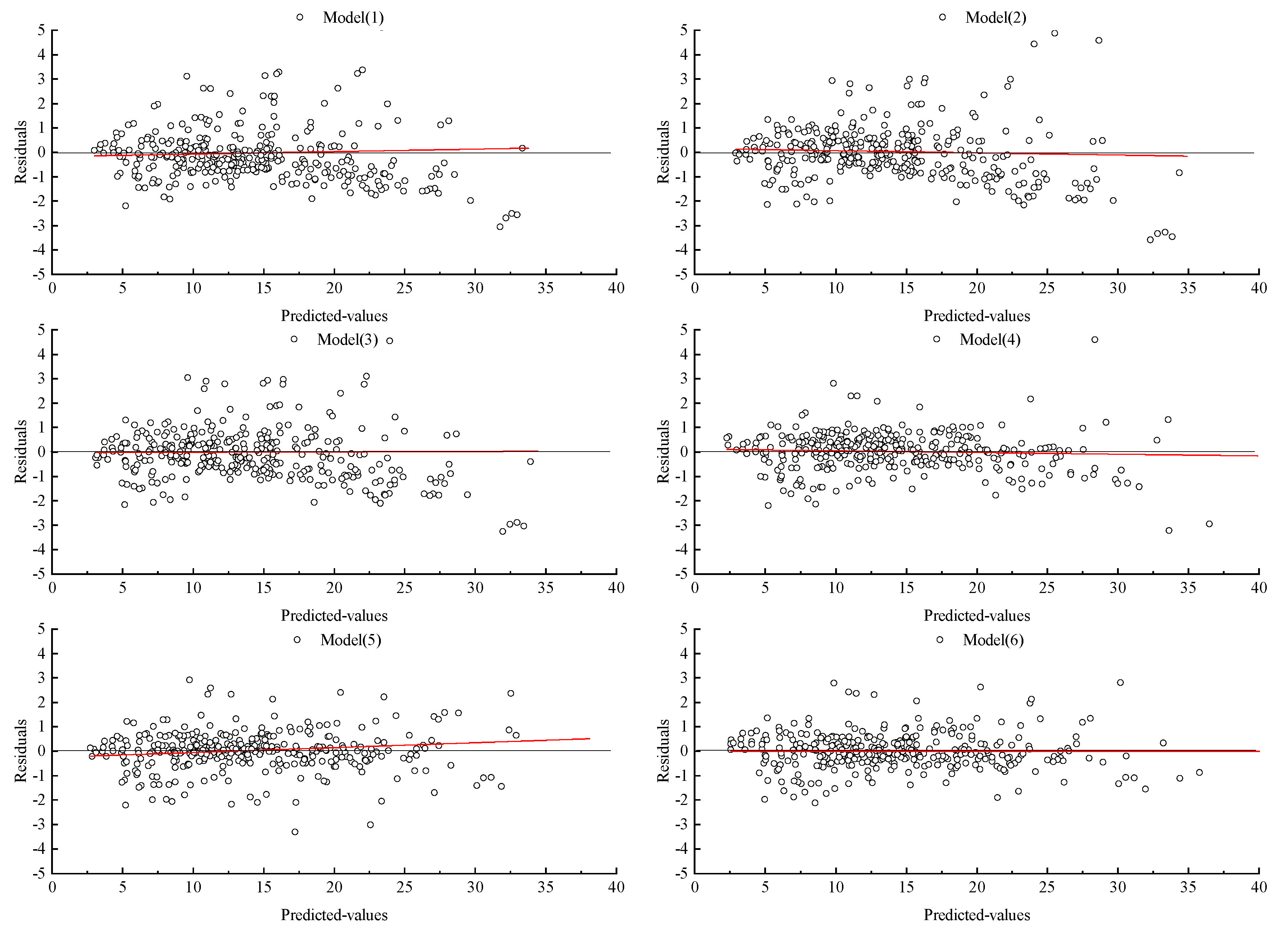
To more comprehensively evaluate the fitting effect of the TLS data, Figure 3 and Figure 4 plot the residual graphs and trend lines of the six models of both datasets, respectively. The figure shows that both datasets have the high equal variance and unbiased characteristic of model (6), and the residual distribution is more uniform.

Table 5. Test statistics of the taper equation.

Model	TLS Data				Stem Analysis
	Bias/cm	RMSE/cm	R2	P (%)	Bias/cm	RMSE/cm	R2	P (%)
1	2.0072	2.5222	0.8679	97.6835	2.0422	2.5622	0.8659	97.6472
2	1.1989	1.8004	0.9327	98.3307	1.3125	1.9359	0.9234	98.2053
3	1.2110	1.8288	0.9306	98.2961	1.3134	1.9631	0.9213	98.1712
4	0.7950	1.1401	0.9730	98.9377	0.7924	1.2182	0.9697	98.8651
5	0.8555	1.3511	0.9621	98.7412	0.7485	1.2809	0.9665	98.8068
6	0.7206	1.0455	0.9773	99.0014	0.7116	1.1069	0.9750	98.9429

shows the test results of the taper equation. Except for model (5), the R² of the TLS data of the other models as greater than the measured data. The prediction accuracy of the TLS data was more than 97%, and the testing results of the six models were consistent with the fitting effect. Both datasets had the largest R² in model (6), the smallest Bias and RMSE, and the highest accuracy. Therefore, the model (6) among these was selected and used for the next analysis.

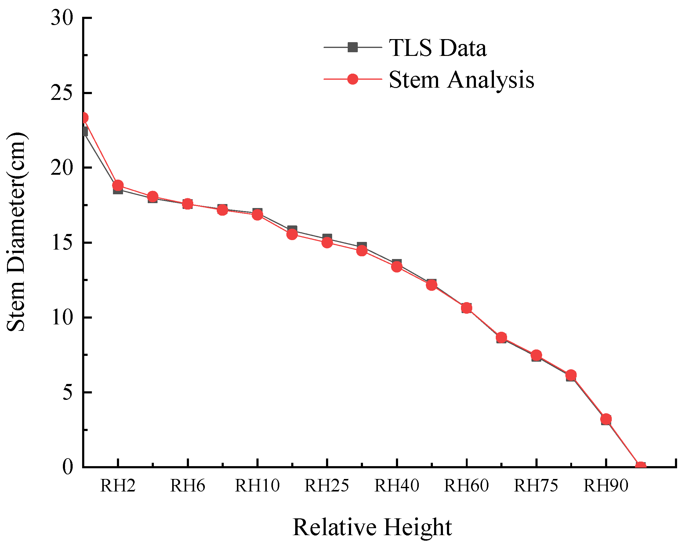
To more clearly describe the effect of the taper equation established by the TLS data, the average values of the DBH and TH extracted from the sample plot were used as the DBH (17.20 cm) and TH (18.64 m) of the simulated tree, and model (6) was used to draw the stem curve of both datasets. As shown in Figure 5, the taper model of TLS basically coincides with the stem analysis. According to the fitting and testing results of stem analysis, the effects of the TLS data are consistent with the stem analysis data, with only slight differences in statistical indicators. Therefore, we believe that TLS data can be used instead of the data from felled trees to establish the taper equation.

3.3. Fitting and Testing of the Taper Models with Different Relative Heights

Since the scanning effect of TLS is easily blocked by branches and leaves, it is difficult to obtain detailed structural information on the upper part of the tree. When the diameter is extracted to RH50, the accuracy is 96.78% and decreases with height. The accuracy of the TLS data will affect the fitting effect of the taper model. Therefore, according to the extraction accuracy mentioned above, this study used diameters from 0 m to relative heights of RH50, RH60, RH70, RH75, RH80, and RH90 to establish the taper equation. The optimal basic taper equation (model 6: Kozak (2002)-II) mentioned above was adopted, and the same method was used for fitting and testing. The results are shown in

Table 6. Fitting and testing of the taper models with different relative heights.

Relative Heights	Fitting Data			Testing Data
	Bias/cm	RMSE/cm	R2	Bias/cm	RMSE/cm	R2	P (%)
0-RH50	0.4603	0.6365	0.9892	0.5685	0.8747	0.9754	99.1421
0-RH60	0.4740	0.6505	0.9890	0.5787	0.8774	0.9768	99.1553
0-H70	0.5043	0.6906	0.9882	0.6148	0.9249	0.9764	99.1193
0-RH75	0.5434	0.7445	0.9870	0.6613	0.9706	0.9765	99.0799
0-RH80	0.5531	0.7553	0.9872	0.6921	1.0081	0.9767	99.0441
0-RH90	0.5500	0.7519	0.9876	0.7206	1.0455	0.9773	99.0014

0-RH50 means that only the diameter data at 0 m, RH2, RH4, RH6, RH8, RH10, RH20, RH25, RH30, RH40, RH50 are used, and the maximum relative height is RH50. The other relative height ranges can be interpreted in a similar manner.

.

The taper model of 0 m-RH60 has the highest accuracy (99.16%), which is 0.15% higher than that obtained using all the data. At 0 m-RH50, the accuracy is high, but there are fewer data representing the shape of the upper stem. At 0 m-RH70, RH75, RH80, and RH90, the accuracy of the model is consistent with the diameter extraction, and both gradually decrease with height.

Based on the accuracy of diameter extraction and model fitting, RH70 is considered to be the best height for TLS to obtain the stem diameter. The extraction accuracy of RH70 is slightly different from RH60 but is much higher than that of RH75 and RH80. As more data are collected from RH70 to RH90, the lower the accuracy of the model is (99.12% at RH70). Therefore, RH75, RH80, RH90 were discarded and the data having 0 m-RH70 diameters were selected for further analyses.

3.4. Sample Plot Mixed Effects Model

3.4.1. Sample Plot Taper Model

According to previous research results, this study used Model 6 (Kozak (2002)-II) and the diameter of the trees in the sample plots at 0 m-RH70 to establish the taper equation. The model parameters and statistics are shown in

Table 7. Fitting parameters and statistics of the sample plot taper model.

Parameter	Parameter Value	Standard Error	t	p-Value	Bias/cm	RMSE/cm	R2
a1	0.9590	0.0193	49.598	<0.0001
a2	1.0682	0.0069	155.304	<0.0001
a3	−0.0473	0.0110	−4.291	<0.0001
a4	0.3377	0.0292	11.555	<0.0001
a5	−0.2760	0.0525	−5.261	<0.0001	0.7663	1.1057	0.9665
a6	0.3814	0.0171	22.312	<0.0001
a7	1.8883	0.2203	8.571	<0.0001
a8	0.0239	0.0011	20.771	<0.0001
a9	−0.2020	0.0182	−11.118	<0.0001

. The t-test shows that the model parameter estimates are all significant (p < 0.0001), and the fitting statistics (R² = 0.9665) indicate that the model could well describe the variation trend of the stem shape of larch.

3.4.2. Mixed Effects Model

Table 8. Comparison of the mixed models with different random effect parameters.

	Parameters	Parameter Number	AIC	BIC	−2Log Likelihood	LRT	p
Basic Model	None	9	16,320.55	16,386.43	16,300.56
Mixed Model	a8	11	15,477.42	15,549.87	15,455.42	845.14	<0.0001
	a6, a9	13	14,068.19	14,153.80	14,042.19	1413.23	<0.0001

lists some of the models with a good fitting of random parameters. It can be seen from the table that the mixed model with random effects is superior to the basic model. When a random parameter a₈ is introduced, the fitting effect of the mixed model is better; a₆ and a₉, as the combination of two random parameters, have a better fitting effect. The likelihood ratio test shows that the models are significantly different from each other. A comprehensive analysis considering the tree effect with two random parameter combinations (a₆ and a₉) is the best mixed model.

3.4.3. Heteroscedasticity and Autocorrelation of Mixed Model Errors

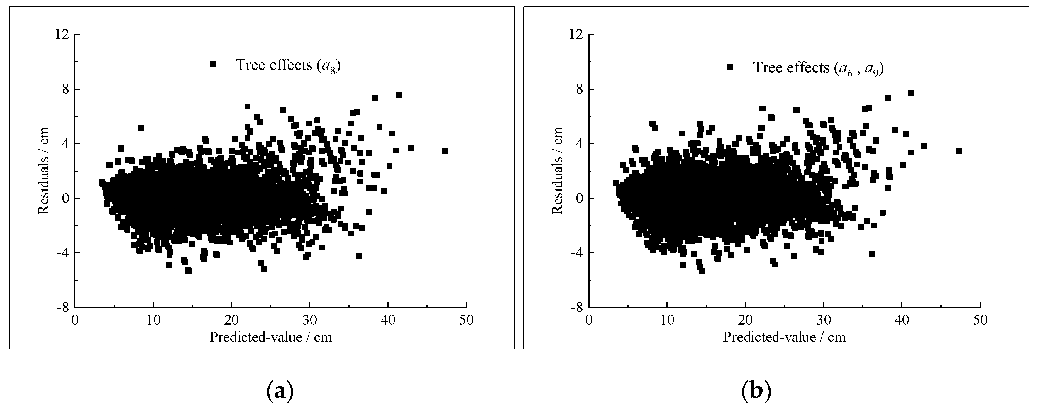
In this study, the heteroscedasticity of the error was judged by the residual distribution diagram. The residual in Figure 6 shows the trend of the random distribution, which indicates that the errors of the mixed model have no heteroscedasticity. First-order autoregressive structure AR (1) is used to solve the autocorrelation problem of diameters measured on the same tree.

Table 9. Comparisons of mixed models with an autocorrelation matrix for larch plantation.

Model	Time Series Correlation Structure	Parameter Number	AIC	BIC	−2Log Likelihood	LRT	p
Mixed (a8)	None	11	15,477.42	15,549.87	15,455.42
	AR(1)	12	13,479.63	13,558.66	13,455.63	1999.79	<0.0001
Mixed (a6,a9)	None	13	14,068.19	14,153.80	14,042.19
	AR(1)	14	13,258.57	13,333.01	13,212.81	829.38	<0.0001

shows that when AR (1) is added, the three evaluation indexes and likelihood ratio confirmed that the AR (1) significantly improved the fitting accuracy of the mixed-effect model.

3.4.4. Mixed Model Evaluation

Table 10. Parameters, variance estimates and fitting statistics of different models.

	Parameter	Basic Model	Mixed Model
			(a8)	(a6,a9)
	a1	0.9590	0.8474	0.9288
	a2	1.0682	1.0596	1.0469
	a3	−0.0473	0.0064	−0.0129
Parameter	a4	0.3377	0.4409	0.5763
	a5	−0.2760	−0.0501	−0.0346
	a6	0.3814	0.3136	0.3539
	a7	1.8883	0.8981	−0.2115
	a8	0.0239	0.0063	0.0024
	a9	−0.2020	−0.0316	0.0357
	σ	36.5198	1.0945	0.7160
Variance components	${\sigma }_i^2$			0.0118
	${\sigma }_j^2$			0.0194
	${\sigma }_{ij}^2$			−0.8250
Time series correlation structure	ρ		0.6661	0.5132
Goodness-of-fit statistics	Bias/cm	0.8039	0.7178	0.5683
	RMSE/cm	1.2245	0.9827	0.7610
	R2	0.9600	0.9736	0.9841

Note: ${\sigma }_i^2$ and ${\sigma }_{ij}^2$ are the variance and covariance parameters for the tree effect; $\sigma$ is the residual variance; and $\rho$ is an autoregressive parameter, $\rho$ > 0.

lists the parameter values and fitting statistics of the basic model and the mixed model with the tree effect. The results show that the R² of the mixed model is greater than that of the basic model, and the Bias and RMSE are both smaller, which indicates that the fitting effect of the mixed model is better than that of the basic model.

3.4.5. Mixed Model Test

The prediction accuracy of the random effect mixed model reached 99.72%, which is higher than that of the basic model and fixed effect model, and the bias was reduced by 0.0249 cm (

Table 11. Validation for the basic and mixed models.

Verification Statistics	Basic Model	Mixed Model
		Fixed Effects	Random Effects
Bias/cm	0.8039	0.8180	0.7790
RMSE/cm	1.2245	1.2459	1.1574
R2	0.9600	0.9589	0.9645
P/%	99.7091	99.7040	99.7244

). This result indicates that the taper model based on the TLS data can be widely used in forestry.

3.5. Application of the Model

3.5.1. Mixed Model Predicts the Stem Diameter

The accuracy (

Table 12. Prediction of the diameter at different relative heights using the taper equation.

Relative Height	TLS Data				Stem Analysis
	Bias/cm	RMSE/cm	R2	P/%	Bias/cm	RMSE/cm	R2	P/%
0 m	1.2904	1.7372	0.9590	94.4294	1.5049	2.4178	0.9190	94.1768
RH2	0.5791	0.8178	0.9833	97.0611	0.7567	0.9860	0.9745	95.9787
RH4	0.5065	0.7205	0.9838	97.6722	0.4660	0.6838	0.9855	97.4916
RH6	0.5626	0.7177	0.9828	97.2212	0.4438	0.6213	0.9872	97.6593
RH8	0.4521	0.6568	0.9851	97.8422	0.4400	0.6246	0.9865	97.6846
RH10	0.3966	0.6102	0.9866	98.1641	0.4388	0.6096	0.9867	97.6425
RH20	0.5015	0.6037	0.9857	96.6956	0.4303	0.5668	0.9875	97.2600
RH25	0.4434	0.5705	0.9871	96.7790	0.5260	0.6112	0.9840	96.3208
RH30	0.4488	0.5511	0.9863	96.6770	0.5108	0.6153	0.9821	96.3955
RH40	0.4169	0.5746	0.9828	96.8288	0.4161	0.5704	0.9822	96.9709
RH50	0.6253	0.7967	0.9591	95.0573	0.5693	0.8132	0.9538	95.5927
RH60	0.7228	0.9152	0.9377	93.9006	0.6553	0.9298	0.9302	94.5820
RH70	1.0094	1.2264	0.8662	89.1886	0.7605	1.0505	0.8871	92.0580
RH75	1.1523	1.4314	0.7848	85.6784	0.8534	1.1415	0.8524	89.5416
RH80	0.8901	1.2358	0.7513	87.6142	0.8565	1.1316	0.7497	87.2974
RH90	-	-	-	-	0.8720	1.1139	0.3358	74.2177

) of the taper equation in deriving the diameter can reach more than 85% (except RH90). Consistent with the variation trend of the TLS extraction accuracy, the lower accuracy of the upper stem is only 74.22% at RH90. In forest inventory assessments, tree crowns and treetops are generally not used for timber production. Therefore, the data obtained using TLS in this study have important practical value.

3.5.2. Volume Estimation by the Mixed Model

The volume predicted by the two methods is very close to the reference value. Method 2 provides better performance (

Table 13. Volume estimation statistics.

	Bias/m3	RMSE/m3	R2	P/%
Method 1	0.0184	0.0327	0.9802	93.4122
Method 2	0.0105	0.0186	0.9933	96.3848

), i.e., the method of nondestructive TLS measurements is suitable for deriving the taper function and stem volume.

4. Discussion

The conventional construction of the taper equation is performed by obtaining data by cutting down trees, which is a waste of time and energy. This research provides a new nondestructive TLS scanning method, which not only provides Woodsfield data for verification but also provides large-scale plot data for modeling. Compared with Sun’s study (applying 198 trees as samples in 8 plots, 16 of which were subjected for stem analysis) [32], this study involved more data (a total of 580 trees in 9 plots, and another 30 were subjected to stem analysis), and this study therefore better represents the actual state. Most studies on the diameter of TLS acquisition are limited to stems with DBHs, while there are few studies on upper TLS acquisition. Xi et al. [21] reported that the occlusion of the crown introduces biases above 12 m in stem form extraction. In this study, the diameters of the relative positions were extracted, which not only reduced the influence of the tree height but also derived the diameters through the taper model.

According to the diameter extraction of different relative heights in the stem analysis, the accuracy of the entire tree decreases with height. Notably, the accuracy at RH75 is less than that at RH80. The study showed that during TLS scanning, due to the influence of wind blowing on the tree or the error in the registration of the station, there are angles or ghosts in the upper part of the stem at different stations. There will be errors in the registration of different stations of point cloud data, which is shown in Figure 2a, and tree heights in this study ranged from RH75 to RH80. The visual error, shown in blue in Figure 2b, may overestimate or underestimate the diameter. At RH75, the tree point clouds are mixed together, so it is not easy to interpret the stem. At RH80, the stem point clouds are separated, which is easy to interpret and has little visual error. At 0.9H, the point cloud density decreases, the stem diameter is difficult to interpret, and the extraction error increases. Beam divergence of the scanner is the key determinate of the increasing error with height. To overcome this problem, we used multiple scans of trees from different perspectives. Xi et al. [21] scanned plots using Leica HDS6100 by the Finnish Geodetic Institute (FGI), and the results showed that the DBH extraction accuracy was 0.97 (r²) and 0.90 cm (RMSE). In our study, the DBH extraction accuracy was 0.9958 (R²) and 0.3726 cm (RMSE). Li Dan et al. [33] used Riegl VZ-400 to scan 5 plots, and the average RMSE of DBH and TH extracted automatically were 2.53 cm and 3.80 m, respectively (lower than ours). In addition, the stand density, crown density, tree height, branch growth condition, understory vegetation, and number and distance of stations will all affect the accuracy.

Internationally, the tree detection rate, stem position, DBH, TH, wood volume, biomass and other forest measurement processes of TLS have reached a high degree of automation [34]. Compared with traditional methods, the DBH and TH are automatically obtained by algorithms, such as Cabo C, where 85% of the DBH deviations are lower than 1 cm and 92% of the TH differences are less than 0.5 m [35]. This study used manual extraction, except for 0 m, and all diameter errors were less than 1 cm. With regard to the quality of the data, the accuracy in this study was higher, but the processing time was longer and the workload was greater. Regardless, the lower portions of the trees are obscured by understory vegetation, as well as other trees and branches, or the lack of scanning points on the treetops.

According to fitting analysis of the three types of taper equations, it was concluded that the variable-exponential taper equation has the highest accuracy, and the segmented taper equation also has a higher accuracy, which is consistent with previous studies. Fitting the basic taper equation, the results indicate that RH70 is the maximum height for TLS to obtain diameter data. In our view, this position has higher accuracy and can reduce the processing time of redundant data.

Relevant studies have shown the predictive ability of the random effect mixed model preference at tree levels [36]; therefore, this study only considered the tree effect but not the plot effect. A stem taper is susceptible to the tree crown characteristics. Whether it is a segmented taper equation [12] or a variable-exponential taper equation, the mixed model with the tree effect can better manage the hierarchical structure of the data. Another innovation of this study is that TLS was entirely used to obtain the diameters, and TH was used to establish a taper equation mixed model, which was obtained without cutting down trees. The RD1000 was also adopted for non-destructive tree measurement, as it had the largest mutation when the relative height was 0.64–0.8, similar to the results of our previous study (RH75) [37]. Sun et al. [32] used a modified Schumacher equation to fit the Populus L. taper equation of the TLS, which yielded a fitting R² = 0.96, which is similar to that of the basic model in our study but lower than that of the mixed model (R² = 0.98). Other studies have recommended that, as a variable for calculating volume, the cross-section area exhibits better performance than the diameter [38]. The prediction quality of the taper and volume model can also be calibrated with an additional diameter measured between 40% and 60% of the total tree height [36,39,40]. When the diameter of the calibration measurement is 7 m, the average deviation of the merchantable volume is only 0.63% [41].

5. Conclusions

In this study, TLS was used to obtain forest parameters, a small amount of field data was used to verify its accuracy, and a mixed model was established to improve the prediction effect of the taper equation. The results show that nondestructive TLS measurements are suitable for deriving stem diameters and trunk volumes; they are feasible for forest investigations.

The optimal height of diameter extraction is RH70; this accuracy meets the requirements of forestry surveys, and also reduces much of the point cloud data processing work. If the extracted height is too high, the diameter accuracy of the upper tree will be low, which will cause a significant amount of redundant data. Conversely, if the extracted height is too low, the amount of data acquired will be too low, which will affect the stem curve. In addition, the amount and accuracy of the data will affect the fitting of the taper model, which in turn affects the simulation of the stem curve and volume estimation.

The taper equation model based on both datasets has a better fitting effect and higher accuracy (model (6): R² > 0.97, P > 98.94%), so the optimal basic taper equation was selected to establish the mixed model with the tree effect. The accuracy of the mixed model based on the tree effect reached 99.72%. The mixed model can accurately predict the diameter of the upper stem, which resolved the problem of the occlusion by the crown. The diameter accuracy derived from the mixed model reached 99%, and the bias was <1.5 cm; it also had high accuracy in estimating the volume of the stem.

The taper equation established by TLS data has typical representativeness and good practicability. In future field measuring work, this method can be used to conduct high-accuracy forest surveys without cutting trees.

References

- Li, F.; Liu, H.; Lu, Y.; Yuan, Y. Compatible Stem Taper and Volume Ratio Equation for Korean Pine. J. For. Res. 1996, 7, 1–6. [Google Scholar]
- Meng, X. Studies of Taper Equations and the Table of Merchantable Volumes. J. Nanjing Technol. Coll. For. Prod. 1982, 122–133. [Google Scholar]
- Jiang, L.; Liu, R. A Stem Taper Model with Nonlinear Mixed Effects for Dahurian Larch. Sci. Silvae Sin. 2011, 47, 101–106. [Google Scholar]
- Kozak, A. My Last Words on Taper Equations. For. Chronicl 2004, 80, 507–515. [Google Scholar] [CrossRef] [Green Version]
- Sharma, M.; Zhang, S.Y. Variable-Exponent Taper Equations for Jack Pine, Black Spruce, and Balsam Fir in Eastern Canada. For. Ecol. Manag. 2004, 198, 39–53. [Google Scholar] [CrossRef]
- Lejeune, G.; Ung, C.H.; Fortin, M.; Guo, X.J.; Lambert, M.C.; Ruel, J.C. A Simple Stem Taper Model with Mixed Effects for Boreal Black Spruce. Eur. J. For. Res. 2009, 128, 505–513. [Google Scholar] [CrossRef] [Green Version]
- Li, C.; Tang, S. The Basal Area Model of Mixed Stands of Larix olgensis, Abies nephrolepis and Picea jezoensis Based on Nonlinear Mixed Model. Sci. Silvae Sin. 2010, 46, 106–113. [Google Scholar]
- Doyog, N.D.; Lee, Y.J.; Lee, S.J.; Kang, J.T.; Kim, S.Y. Compatible Taper and Stem Volume Equations for Larix kaempferi (Japanese Larch) Species of South Korea. J. Mt. Sci. 2017, 14, 1341–1349. [Google Scholar] [CrossRef]
- Menéndez-Miguélez, M.; Canga, E.; álvarez-álvarez, P.; Majada, J. Stem Taper Function for Sweet Chestnut (Castanea sativa Mill.) Coppice Stands in Northwest Spain. Ann. For. Sci. 2014, 71, 761–770. [Google Scholar] [CrossRef]
- Sharma, M.; Parton, J. Modeling Stand Density Effects on Taper for Jack Pine and Black Spruce Plantations Using Dimensional Analysis. For. Sci. 2009, 55, 268–282. [Google Scholar]
- Tang, C. Growth Modeling and Site Quality Evaluation for Betula Alnoides Plantations. Ph.D. Dissertation, China Academy of Forestry, Beijing, China, 2017. [Google Scholar]
- Jiang, L.C.; Jiang, Y.H. Modeling Effects of Crown Characteristics on Stem Taper of Dahurian Larch Using Mixed Model. J. Beijing For. Univ. 2014, 36, 10–14. [Google Scholar]
- Cai, J.; Pan, W.; Wang, B.; Huang, H. Study on Effect of Stand Density on Tree Stem Form of Slash Pine. Guangdong For. Sci. Technol. 2006, 22, 6–10. [Google Scholar]
- Dassot, M.; Constant, T.; Fournier, M. The Use of Terrestrial LiDAR Technology in Forest Science: Application Fields, Benefits and Challenges. Ann. For. Sci. 2011, 68, 959–974. [Google Scholar] [CrossRef] [Green Version]
- Hilker, T.; Leeuwen, M.V.; Coops, N.C.; Wulder, M.A.; Newnham, G.J.; Jupp, D.L.B.; Culvenor, D.S. Comparing Canopy Metrics Derived from Terrestrial and Airborne Laser Scanning in a Douglas-Fir Dominated Forest Stand. Trees 2010, 24, 819–832. [Google Scholar] [CrossRef]
- Henning, J.G.; Radtke, P.J. Detailed Stem Measurements of Standing Trees from Ground-Based Scanning LIDAR. For. Sci. 2006, 52, 67–80. [Google Scholar]
- Liang, X.; Kankare, V.; Yu, X.; Hyyppa, J. Automated Stem Curve Measurement Using Terrestrial Laser Scanning. IEEE Trans. Geosci. Remote Sens. 2013, 52, 1739–1748. [Google Scholar] [CrossRef]
- Liu, L.; Pang, Y.; Li, Z.; Xu, G.; Zheng, G. Retrieving Structural Parameters of Individual Tree through Terrestrial Laser Scanning Data. J. Remote Sens. 2014, 18, 365–377. [Google Scholar]
- Xing, W. Study of Forest TLS Point Cloud Data Automatic Registration Algorithm. Master’s Thesis, Northeast Forestry University, Harbin, China, 2018. [Google Scholar]
- Bauwens, S.; Bartholomeus, H.; Calders, K.; Lejeune, P. Forest Inventory with Terrestrial LiDAR: A Comparison of Static and Hand-Held Mobile Laser Scanning. Forests 2016, 7, 127. [Google Scholar] [CrossRef] [Green Version]
- Xi, Z.; Hopkinson, C.; Chasmer, L. Automating Plot-Level Stem Analysis from Terrestrial Laser Scanning. Forests 2016, 7, 252. [Google Scholar] [CrossRef] [Green Version]
- Yang, Y.; Zhang, S.; Lin, W. Stem Taper Function of Betula Platyphylla with Terrestrial 3D Laser Scanning. J. Northeast For. Univ. 2018, 046, 58–63. [Google Scholar]
- Rodriguez, F.; Lizarralde, I.; Fernández-Landa, A.; Condés, S. Non-Destructive Measurement Techniques for Taper Equation Development: A Study Case in the Spanish Northern Iberian Range. Eur. J. For. Res. 2014, 133, 213–223. [Google Scholar] [CrossRef]
- Li, F. Forest Mensuration, 4th ed.; China Forestry Press: Beijing, China, 2019; p. 205. ISBN 978-7-5219-0182-5. [Google Scholar]
- Jiang, L.C.; Li, F.R.; Liu, R.L. Compatible Stem Taper and Volume Models for Dahurian Larch. J. Beijing For. Univ. 2011, 33, 1–7. [Google Scholar]
- Kozak, A.; Munro, D.D.; Smith, J.H.G. Taper Functions and Their Application in Forest Inventory. For. Chron. 1969, 45, 278–283. [Google Scholar] [CrossRef]
- Max, T.A.; Burkhart, H.E. Segmented Polynomial Regression Applied to Taper Equations. For. Sci. 1976, 22, 283–289. [Google Scholar]
- Zeng, W.; Liao, Z. A Study on Taper Equation. Sci. Silvae Sin. 1997, 33, 127–132. [Google Scholar]
- Pinheiro, J.; Bates, D. Model Building for Nonlinear Mixed-Effects Models; Department of Statistics University of Wisconsin–Madison: Madison, WI, USA, 1994. [Google Scholar]
- Davidian, M.; Giltinan, D.M. Nonlinear Models for Repeated Measurement Data: An Overview and Update. J. Agric. Biol. Environ. Stat. 1995, 8, 387–419. [Google Scholar] [CrossRef]
- Vonesh, E.F.; Chinchilli, V.M. Linear and Nonlinear Models for the Analysis of Repeated Measurements. J. Biopharm. Stat. 1996, 18, 595–610. [Google Scholar]
- Sun, Y.; Liang, X.; Liang, Z.; Welham, C.; Li, W.; Jokela, E.J. Deriving Merchantable Volume in Poplar through a Localized Tapering Function from Non-Destructive Terrestrial Laser Scanning. Forests 2016, 7, 87. [Google Scholar] [CrossRef]
- Li, D.; Pang, Y.; Yue, C.; Zhao, D.; Xu, G. Extraction of Individual Tree DBH and Height Based on Terrestrial Laser Scanner Data. J. Beijing For. Univ. 2012, 34, 79–86. [Google Scholar]
- Liang, X.; Hyypp, J.; Kaartinen, H.; LehtomKi, M.; PyRL, J.; Pfeifer, N.; Holopainen, M.; Brolly, G.; Francesco, P.; Hackenberg, J. International Benchmarking of Terrestrial Laser Scanning Approaches for Forest Inventories. ISPRS J. Photogramm. Remote Sens. 2018, 144, 137–179. [Google Scholar] [CrossRef]
- Cabo, C.; Ordóez, C.; López-Sánchez, C.A.; Armesto, J. Automatic Dendrometry: Tree Detection, Tree Height and Diameter Estimation Using Terrestrial Laser Scanning. Int. J. Appl. Earth Obs. Geoinf. 2018, 69, 164–174. [Google Scholar] [CrossRef]
- Arias-Rodil, M.; Castedo-Dorado, F.; Cámara-Obregón, A.; Diéguez-Aranda, U. Fitting and Calibrating a Multilevel Mixed-Effects Stem Taper Model for Maritime Pine in NW Spain. PLoS ONE 2015, 10, e0143521. [Google Scholar] [CrossRef] [PubMed]
- Marchi, M.; Scotti, R.; Rinaldini, G.; Cantiani, P. Taper Function for Pinus Nigra in Central Italy: Is a More Complex Computational System Required? Forests 2020, 11, 405. [Google Scholar] [CrossRef] [Green Version]
- Gregoire, T.G.; Schabenberger, O.; Kong, F. Prediction from an Integrated Regression Equation: A Forestry Application. Biometrics 2000, 56, 414–419. [Google Scholar] [CrossRef]
- Cao, Q.V.; Wang, J. Evaluation of Methods for Calibrating a Tree Taper Equation. For. Sci. 2015, 61, 213–219. [Google Scholar] [CrossRef] [Green Version]
- Sabatia, O.C.; Burkhart, E.H. On the Use of Upper Stem Diameters to Localize a Segmented Taper Equation to New Trees. For. Sci. 2015, 61, 411–423. [Google Scholar] [CrossRef]
- Adamec, Z.; Adolt, R.; Drápela, K.; Závodsk, J. Evaluation of Different Calibration Approaches for Merchantable Volume Predictions of Norway Spruce Using Nonlinear Mixed Effects Model. Forests 2019, 10, 1104. [Google Scholar] [CrossRef] [Green Version]
Figure 1.
Diameter extraction position of a tree. (a) The height of the diameter extraction position; RH represents relative height. Example: RH40 represents the relative height in the 40th percentile or percentile height; (b) a larch colored by height; (c) the height (m) represented by different colors in (b).
Figure 2.
Multi-station stem point cloud after registration. (a) Different stations near RH75 of the tree point clouds; (b) segmentation (RH75) of the point clouds displayed in 2D. Pink represents the point clouds to be diameter-fitted.
Figure 3.
Model residual distribution of the TLS data.
Figure 4.
Model residual distribution of the measured stem analysis data.
Figure 5.
Taper model of the TLS data and stem analysis data for a single tree.
Figure 6.
Mixed model residuals. (a) Introduce a residual distribution diagram of a random parameter (); (b) consider the residual distribution diagram with two random parameter combi-nations ().