Article

Ecological Niches and Suitability Areas of Three Host Pine Species of Bark Beetle Dendroctonus mexicanus Hopkins

by
Fátima M. Méndez-Encina
1,
Jorge Méndez-González
1,*,
Rocío Mendieta-Oviedo
1,
José Ó. M. López-Díaz
1 and
Juan A. Nájera-Luna
2
1
Departamento Forestal, Universidad Autónoma Agraria Antonio Narro, Saltillo 25315, Mexico
2
Instituto Tecnológico de El Salto, El Salto 34942, Mexico
*
Author to whom correspondence should be addressed.
Forests 2021, 12(4), 385; https://doi.org/10.3390/f12040385
Submission received: 29 January 2021 / Revised: 11 March 2021 / Accepted: 12 March 2021 / Published: 24 March 2021
(This article belongs to the Section Forest Ecology and Management)

Abstract

:
Bark beetles are a natural part of coniferous forests. Dendroctonus mexicanus Hopkins is the most widely distributed and most destructive bark beetle in Mexico, colonizing more than 21 pine species. The objectives of this study were to generate ecological niche models for D. mexicanus and three of its most important host species, to evaluate the overlap of climate suitability of the association Dendroctonus–Pinus, and to determine the possible expansion of the bark beetle. We used meticulously cleaned species occurrence records, 15 bioclimatic variables and ‘kuenm’, an R package that uses Maxent as a modeling algorithm. The Dendroctonus–Pinus ecological niches were compared using ordination methods and the kernel density function. We generated 1392 candidate models; not all were statistically significant (α = 0.05). The response type was quadratic; there is a positive correlation between suitability and precipitation, and negative with temperature, the latter determining climatic suitability of the studied species. Indeed, a single variable (Bio 1) contributed 93.9% to the model (Pinus leiophylla Schl. & Cham). The overlap of suitable areas for Dendroctonus–Pinus is 74.95% (P. leiophylla) and on average of 46.66% in ecological niches. It is observed that D. mexicanus begins to expand towards climates not currently occupied by the studied pine species.

1. Introduction

Temperate forests cover 15% of the world’s land [1,2]. In Mexico, they cover 13% the country’s territory [3]. Dominated by the genus Pinus, they are especially restricted to mountainous areas, between elevations from 1500 to 4000 m [4], having an affinity for cold temperate climates. These forests contain 49 of the 120 pine species described [5], reaching one of the highest diversities worldwide. Pine forests are of great economic importance for the country. From an ecological perspective, they contribute to regulate global climate acting as CO2 sinks [6]. However, the accumulation of greenhouse effect gases in the atmosphere, caused mainly by human activity, has caused an increase of 0.87 °C in the last 10 years [7]. This trend is occurring more rapidly than had been predicted and could have significant effects on adaptations of living organisms.
Coexisting naturally with conifer species are species of the genus Dendroctonus Erichson, 1836, called bark beetles [8,9]. The genus includes 19 species and one subspecies, of which 17 are found in North and Central America and only two in Asia and Europe [8]. But only a small percentage of the more than 6000 bark beetles found worldwide are capable of causing significant economic damage [10]. Their name comes from Dendro (tree) and tonus (destroyer) [11]; they belong to the Curculionidae family and play a critical role in the dynamics of coniferous forests [12,13]. They vary in size from 0.1 to 6 mm and are endophytes; that is, they dig galleries under the bark of live trees to feed on the phloem [1].
Twelve of the 19 known species of bark beetles are found in Mexico [8,14]. Dendroctonus mexicanus Hopkins is the most widely distributed in the country [14] and the most destructive. Because of the irreversible damage it causes to coniferous forests, it is considered the most important species [15]. It is characterized by high polyphagia, colonizing over 21 species of pine. Pinus leiophylla Schl. & Cham., Pinus teocote Schiede ex Schltdl. and Pinus devoniana Lindley are the preferred species and those of the highest incidence percentage [14].
To manage the future of a country’s forests, it is necessary to determine the impact of climate change on species distribution. Niche-based, correlative species distribution models (hereafter SDMs) have been widely used to predict the potential changes in species distributions under climate change scenarios [16,17,18]. Developing an SDM requires previous knowledge of the conceptual framework [19,20,21], ecological assumptions on which to base species distribution [16,22,23], and of the performance of modeling algorithms [24,25]. Modeling requires records (presence/absence) of the species, predictive variables (e.g., bioclimatic [26], topographic [27], soils [28], among others), and of course, the algorithm. In other words, species distribution is determined by three limiting factors: the geographical region that has been accessible to the species over a given period of time «M», abiotic conditions «A» and biotic interactions «B», simplified in the «BAM» diagram [29]. Predictive mapping results in a spatially explicit “wall-to-wall” prediction of species distribution or habitat suitability [24]. If the fit is good, it is possible to identify the species environmental tolerance and transfer the model in time or space [22]. Although there are several modeling algorithms, it has been demonstrated that Maxent performs better than standard methods; it is one of the most efficient and, therefore, the most widely used [25].
Climate change has made us reflect on possible species re-distribution. Effort is required to understand the dynamics of ecological niches of two or more species (e.g., niche shifts, niche conservatism and niche similarity). A niche is defined as the set of environments suitable to a species [30]. The development of ecological niche models (hereafter ENMs) makes it possible to quantify niche overlap of species, but also shift, stability, centroid and niche unfilling [20,31]. Some authors [18] have shown that due to the effects of climate change, especially temperature, D. mexicanus could modify its distribution towards higher latitudes and altitudes.
Species suitability models have been used to many ends, commonly for conservation and biodiversity plans. However, for the case of the genus Pinus in Mexico, they are not of much use if models of climate suitability of the genus Dendroctonus are not considered since they coexist partially or totally sharing geographical (G) and environmental (E) space. Although much has been gained by generating species suitability models and niche models, it is essential to perform statistical tests to interpret the significance of these patterns. Thus, for the SDM objective in Pinus to be possible, it is necessary to have precise, reliable predictions for suitable areas of Pinus (SAP), free of suitable areas of Dendroctonus (SAD) in order to implement management and conservation strategies integrally.
The objectives of this study were: (i) to generate robust ecological niche and species distribution models for D. mexicanus and three of its most important host species: P. leiophylla, P. teocote and P. devoniana, and with these determine SAP free of SAD; (ii) to evaluate the overlap of climate suitability and of the environmental niche of the association Dendroctonus–Pinus in spaces G and E by means of predictive models and multivariate analysis, and (iii) to determine their climate tolerances using a detailed bioclimatic profile of these species.

2. Materials and Methods

The conifer species P. leiophylla, P. teocote and P. devoniana were selected because they have the highest percentual incidence of bark beetle D. mexicanus attack in Mexico and are the most susceptible species, with 35.6, 13.9 and 9.4%, respectively [14].

2.1. Study Area

The study area differs for each of the species; in general, there are coniferous forests located in the main mountain systems of Mexico, such as the Sierra Madre Occidental (SMOc), Sierra Madre Oriental (SMOr), Trans-Mexico Volcanic Belt (TMVB), Sierra Madre del Sur, Sierra del Norte de Oaxaca, Sierras de Chiapas, and the extremes of Baja California. In these regions annual mean temperatures oscillate between 10 and 20 °C, and annual precipitation is 600 to 1000 mm [4]; altitudes are from 1600 m to a little more than 3000 m (Figure 1).

2.2. Bioclimatic Variables and Selection

Because of the scale of the study area (>200 km), only bioclimatic variables were used (Table 1) [23,32]; these proposed by [33] were re-sampled at a resolution of ∼5 km2. Bio 8, Bio 9, Bio 18 and Bio 19 were excluded from the analysis since, by combining information on precipitation and temperature in the same layer, the resulting predictions were erratic and biased [34].
The selection of the bioclimatic variables was based on four criteria: (1) relative contribution of the variable to the bioclimatic profile of the species [35] was obtained through a principal components analysis (PCA) with the package ‘FactoMiner’ [36], previously extracting from each species occurrence records the value of the 15 bioclimatic variables, making the PCA to the standardized variables and selecting those that contributed most, (2) non-correlated variables (r < 0.8) were determined by a parametric correlation analysis ( α = 0.05 ) of the variables transformed to natural logarithm [25,37,38], (3) variable frequency distribution using the Sturges [39] rule determined how the bioclimatic variable was distributed giving selection priority to those close to a normal distribution or a skewed distribution (left or right) [40], and (4) the predictive capacity of the variable consists of preliminary modeling with individual variables and transferring the model in time and space because it has been demonstrated that climate projections of precipitation of the General Circulation Models (GCMs) are biased at higher latitudes [33], resulting in an overestimation of climate suitability of a species in the same zones. The variables that least overestimate climate suitability of a species were selected. These procedures were carried out in each species.

2.3. Species Occurrence Records and Cleaning

Species occurrence records of each species were downloaded from the Global Biodiversity Information Facility (GBIF) and Red Mundial de Información sobre Biodiversidad (REMIB). Others were obtained by Inventario Nacional Forestal y de Suelos de México (INFyS), published articles and our own fieldwork.
Data cleaning of each specie consisted of eliminating records that were: (1) Outside the geographic range (latitude and longitude), (2) outside the altitudinal range (according to the descriptor of the species), allowing records between quantile 5 and 95 (and/or ±500 m), depending on the species, (3) not precise (equal to or less than three digits), (4) duplicates [17], (5) without author of identification, and (6) outside the ellipse at 99% of a PCA conducted with the package ‘FactoMiner’ [36], using 15 environmental variables and altitude. Spatial autocorrelation between records was then eliminated with the package ‘spThin’ [41], allowing a single record per pixel (∼5 km). If we did not correct for this characteristic, we would have incurred in a biased selection of variables or model coefficients [42].

2.4. Calibration Area

Areas where the species could be observed or that could be explored because of their biological capacity are denoted as «M» in the «BAM» diagram [29]. This was delimited preliminarily in ArcMap v.10.5, applying a 70 km buffer radius to each species occurrence records. In SDM and ENM, the calibration areas should include the complete distribution of the species [20]. If the extension of this area is smaller than the species range, the response function cannot have the predicted form, because of the niche theory [22]. The final delimitation of «M» was achieved with the cleansed records, that is, with those that passed all the cleaning criteria indicated in the previous section.

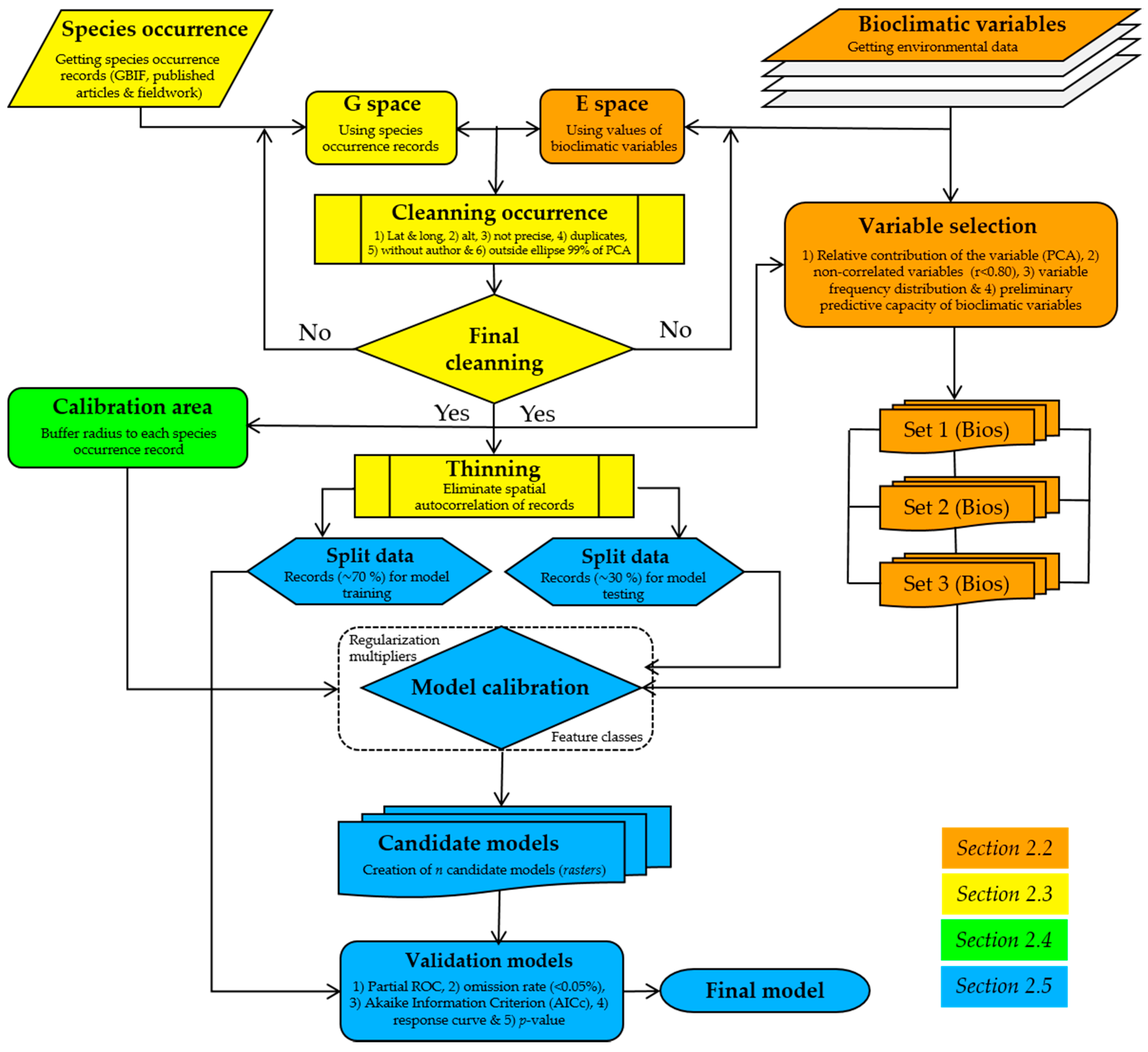
2.5. Model Calibration, Creation, and Evaluation

The model calibration, creation, and evaluation were done in ‘kuenm’, an R package that uses Maxent (maximum entropy) [43] as the modeling algorithm. Maxent has two main modifiable parameters: (1) “regularization multiplier” (β) and (2) “feature classes” such as linear (l), quadratic (q), product (p), threshold (t) and hinge (h). The first is a parameter that adds new constraints; it is a penalty imposed on the model, and the latter corresponds to a mathematical transformation of the different covariates used in the model to allow complex relationships to be modeled [37,44]. For each species, 16 regularization multiplicators were tested (0.1 to 1, 2 to 6, and 10), 29 response types (l, q, p, t, h, lq, lp, lt, lh, qp, qt, qh, pt, ph, th, lqp, lqt, lqh, lpt, lph, qpt, qph, qth, qth, lqpt, lqph, lqth, lpth and lqpth), and three different sets of environmental variables (optional), those that satisfied the selection criteria indicated in Section 2.2.
Modeling was carried out with approximately 70% of the records; with independent data (∼30%), the predictive capacity of the models was evaluated using cross validation [36]. This percentage depends on the availability of independent records of each species used for validation. The output format was of logistical type, which can be interpreted as probability of presence and is recommended if and only if the “regularization multiplier” and “feature classes” [45] are optimized. The resulting models (maps in raster format) represent species suitability values (0–1) [46].
The best fit model was selected according to: (1) the statistic partial ROC (Receptor Operated Curve) [47], (2) the rate of omission <0.05%, (3) the lowest value of the Akaike Information Criterion (AICc) [19,48,49], (4) species response curves to the environmental gradients [37], and (5) statistical significance of the model, p-values [19]. Here, the partial ROC was used instead of the area under the ROC curve (AUC) because the latter is not a good measure of fit in ENM [47,50]. Statistical significance was determined by a bootstrap resampling of 50% of testing data.
To reduce bias, the final selected model was represented by the mean of 10 repetitions, with which prediction uncertainty was obtained. The jackknife tests and the response curves to bioclimatic variables were implemented in ‘kuenm’ [43] to determine the variable’s contribution to the model. The process for generating the climate suitability model of the species is shown in Figure 2.

2.6. Model Stratification

The final continuous model of probability (suitability) of each species was classified in three levels or strata: low, medium and high suitability. To this end, 5000 points were distributed randomly over the suitability model; from these points their value was extracted. Later, in R with the package ‘stratifyR’ [51], the thresholds of each stratum were calculated following the method of Khan et al. (2002) [52], Khan et al. (2008) [53] and Khan et al. (2015) [54]. This method determines the Optimum Strata Boundaries (OSB) and Optimum Sample Sizes (OSS) for the study variable, using the best-fit frequency distribution of a survey variable. It formulates the problem of determining the OSB as a mathematical programming problem, which is solved using a dynamic programming technique, using Neyman Allocation assuring minimum intra-stratum variance and maximum inter-stratum variance.

2.7. Bark Beetle-Free Areas

The final suitability models of each species were converted into binary maps in ArcMap v.10.5 to represent climate suitability-non-suitability. This was done by reclassifying the suitability to 1 and 0; the value of one (1) was assigned to suitability comprehended between the minimum value of the second stratum (calculated in the previous section) and that of maximum suitability, while the value of zero (0) corresponded to the rest of the suitability. The binary maps were manipulated using ‘raster algebra’ of each pair of species (PinusD. mexicanus), and SAP free of SAD were calculated. The procedures based on spatial predictions of climate suitability (also called ENMs), besides estimating SAP–SAD [49], allow quantifying changes and niche overlap of two or more species in G space [20].

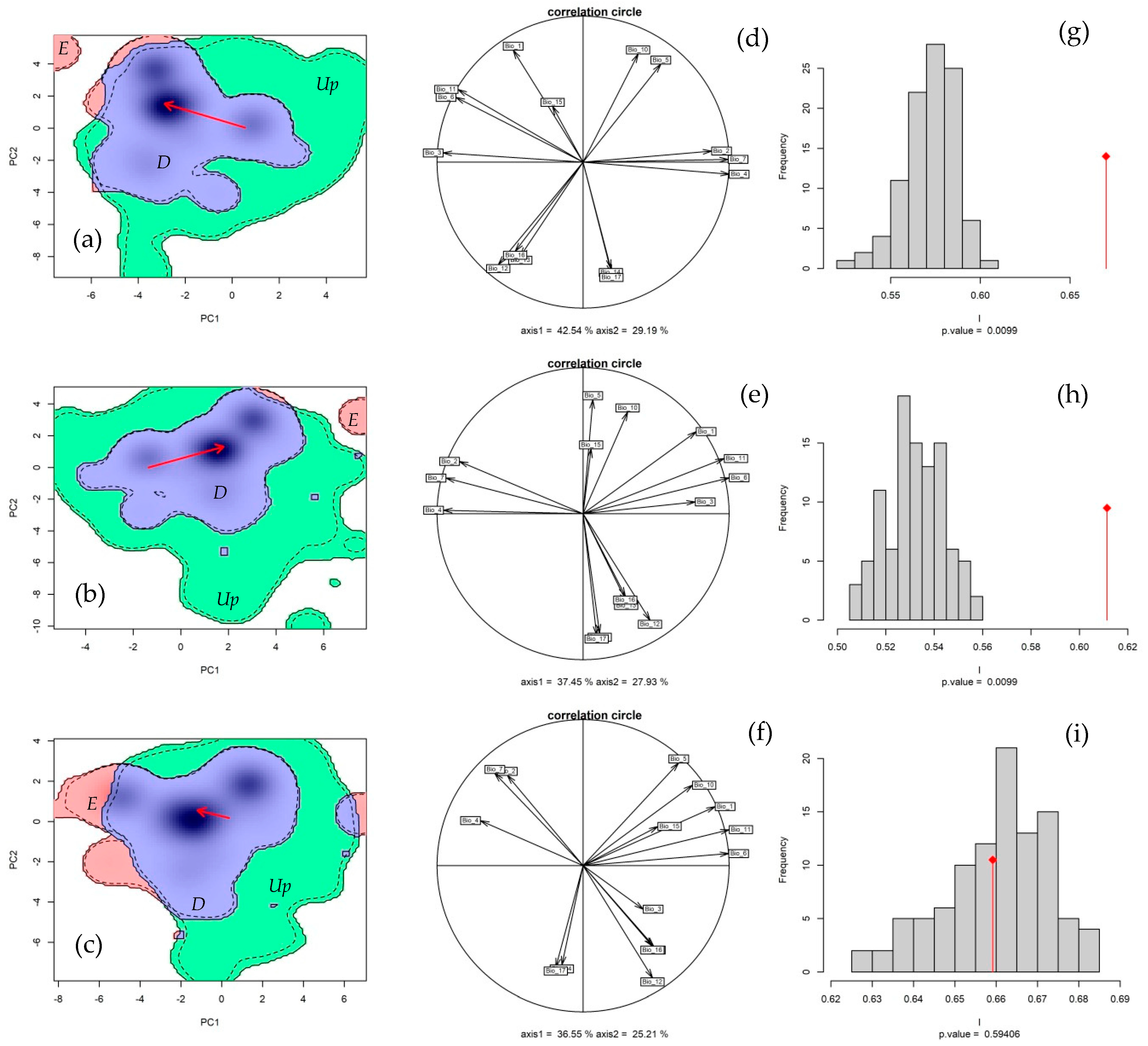
2.8. Quantifying Niche Similarity

Similarity between the Dendroctonus and Pinus niches was calculated with two indexes introduced by Warren et al. (2008) [31]: Schoener’s (1968) [55] D and a measure derived from Hellinger’s distance called I using ordination methods (PCA) and the 15 bioclimatic variables for each species [20] (Table 1). This method is the most precise [56] and the most recommended [20,57]. Both similarity measures range from 0, when species predicted environmental tolerances do not overlap at all, to 1, when overlap is total. Niche comparisons were made relative to the entire niche of the species, pooled from the two ranges [20,31], under the hypothesis of niche conservatism of the genus Pinus; it is known that it was established ∼145 million years ago in the lower Cretaceous [58], and the bark beetle as an invasive species. A kernel density function (standard smoothing parameters) was applied to determine the ‘smoothed’ density of occurrences in each cell in the environmental space for each dataset; the use of a kernel smoother makes the process of moving from G space to multivariate E space, independent of both sampling and resolution in environmental space. The shift of the middle position from centroid of the niche between the species of bark beetle with the pine species was calculated with the C metric, using Euclidian distance [20]. This analysis was performed with the package ‘ecospat’ [59]. All the packages mentioned in this study were run in R 3.6.3 [60].

3. Results

3.1. Generalities

A total of 283, 3648, 2209 and 772 species occurrence records were collected for D. mexicanus, P. leiophylla, P. teocote and P. devoniana, subtracting for the modeling and validation 86, 900, 736 and 255 (30.39, 24.67, 33.32 and 33.03%); that is, up to 75.33% of the P. leiophylla records were eliminated, because they did not meet the established cleaning criteria (Section 2.3).
The PCA performed to select the variables by their contribution, explained 67.63, 73.48, 65.60 and 64.10% for the different species (Table 1). This analysis is statistically valid when the variables correlate with each other (>0.6). The Kaiser–Meyer–Olkin (KMO) index indicated that the global correlation of the PCA was 0.68, 0.71, 0.72, and 0.65, respectively. The results show that in the four species, the variables derived from temperature (Bio 1–Bio 11) are those that most contributed; variable 16 (Precipitation of Wettest Quarter, mm) is that which least contributed (Table 1). There are variables (e.g., Bio 12 and Bio 13, for the species D. mexicanus) that contribute significantly in the PCA (Table 1). However, they were not selected because they presented a bimodal distribution.

3.2. Generated Models and Their Statistics

A total of 1392 candidate models were generated for each species (Table 2). It is notable that not all the models were statistically significant (α = 0.05), registering 99.4% for D. mexicanus, 53.5% for P. leiophylla, 99.9% for P. teocote and only 9.5% for P. devoniana (Table 2), using the default parameters in Maxent does not necessarily produce the best model [61] (see Appendix A). The type of response that prevailed in the selected models was quadratic (Table 2). No linear response model was selected in any case. The algorithm implemented in ‘kuenm’ [43] selected the best regulating multiplier in each species varied from 2 (D. mexicanus and P. devoniana) to 5 (P. leiophylla).
Fewer than 20% of the 1392 models generated passed the omission rate (false negative predictions) established (0.05%); indeed, none satisfied in the species P. leiophylla, having to increase the established value to 0.07% to select the model. Only one model (0.07% of the total) passed all the criteria established in Section 2.5 (Table 2) in D. mexicanus and P. devoniana.

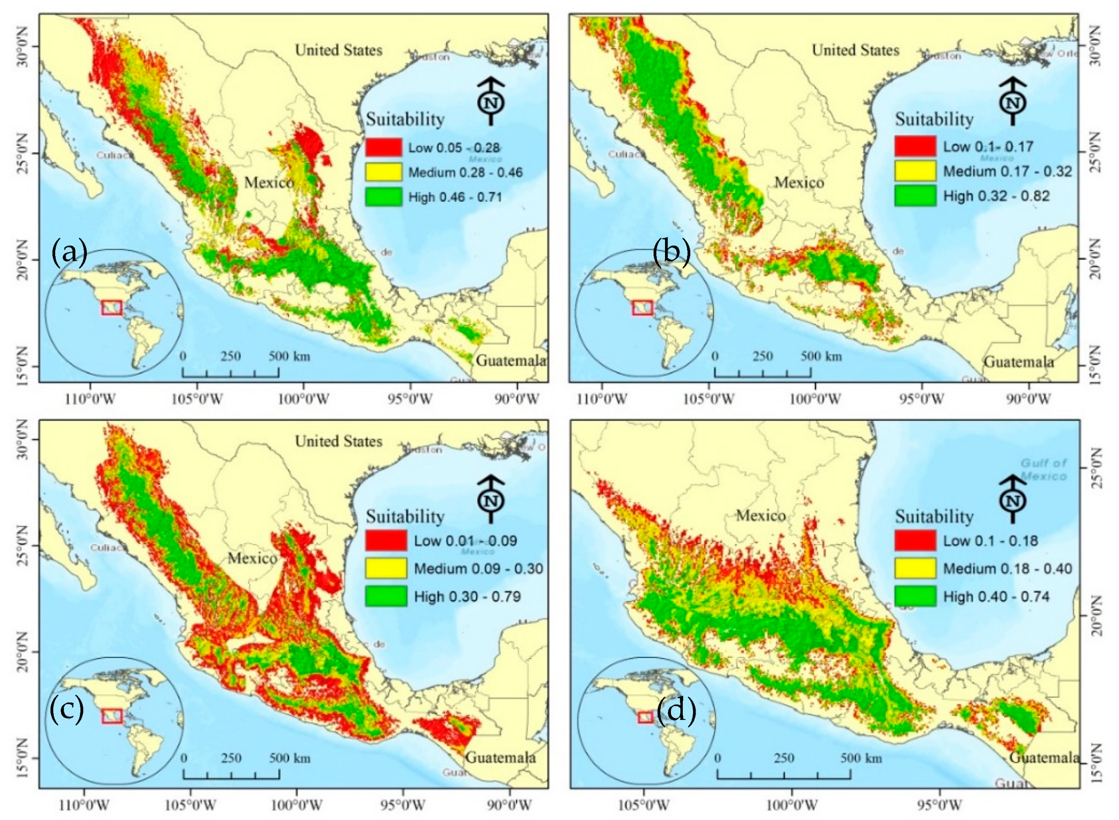
3.3. Species Suitability Areas

In no case did climate suitability reach the maximum value (1), varying from 0.01 (P. teocote) to 0.82 (P. leiophylla). Suitability takes on different forms, triangular in D. mexicanus and P. devoniana with parameters a = 0.001 and 0.001; b = 0.732 and 0.795; c = 0.518 and 0.01, respectively. Gamma distribution in P. leiophylla and P. teocote had values of k = 0.702 and 0.526; λ = 3.082 and 3.728, respectively. The OSBs varied in each species and not in the same amplitude, showing that variance differs in all the spectrum of species climate suitability. For this reason, stratification should obey a statistical technique rather than stratify by proportions, assuring minimum and maximum intra-stratum variance among them.
It is estimated that the area of high suitability in Mexico is 234,649.1, 212,497.4, 177,904.8 and 159,630.4 km2 for D. mexicanus, P. leiophylla, P. teocote and P. devoniana (Figure 3a–d). Except for P. teocote (Figure 3c), high suitability represents that largest part of «M», from 39.89% (P. devoniana, Figure 3d) to 47.85% (P. leiophylla, Figure 3b). The predicted area of suitability for a species is not dependent on the number of registers. Maxent uses presence records to model climate suitability. During this process, the algorithm generates “pseudo absences” where the species is not present. This helps to improve the predictions of the current distribution of the species.

3.4. Bioclimatic Profile

The ‘kuenm’ algorithm selected the set of variables (Table 3) that showed the best predictive capacity, validated with the set of independent records of the species. The sets comprised different numbers of variables, from three (P. leiophylla) to seven (P. teocote). Like the PCA, the jackknife tests showed that the variables derived from temperature (Bio 1–Bio 11) contribute more than 80% to explain the bioclimatic profile of the species (Table 3), especially, the representatives of extreme values. In D. mexicanus and P. leiophylla a single variable contributes significantly to the species bioclimatic profile, 87.8% (Bio 10) and 93.9% (Bio 1), respectively. The average coefficient of variation of the variables that most contribute to the bioclimatic profile of each species (Bio 10, Bio 1, Bio 10 and Bio 11, Table 3) is 14.3%, indicating that the predictors selected by both PCA (preselection of variables) and the ‘kuenm’ algorithm adequately represent the species bioclimatic profile. Only one variable (Bio 6, in P. teocote) experienced high variability (198.9%) but contributes to the bioclimatic profile with only 15.6% (Table 3).

3.5. Climatic Suitability of Pine Species, Free of Bark Beetle Suitability Areas

From the total suitable area predicted for P. leiophylla (444,100.4 km2), P. teocote (729,358.3 km2), and P. devoniana (400,142.8 km2) (Figure 3b–d) and by obtaining SAP–free of SAD of each PinusDendroctonus pair (Section 2.7), we found that only 92,995.2, 11,737.4 and 55,964.8 km2, respectively, are free of suitable bark beetle areas. For P. teocote, of the total of the suitable areas, only 3.02% is left.
Despite the wide distribution of P. leiophylla and P. teocote (Figure 3b–c), SAP–free of SAD are observed only in a northern part of the SMOc (Figure 4a,b), where there is a larger number (seven) of bark beetle species [13], in a compact form for the first pine species P. leiophylla and disperse for the second P. teocote, but inexistent in lower latitudes of the species distribution. In P. devoniana (Figure 4c), the SAP–free of SAD are observed discontinuously over the entire area of its distribution. In all cases, these areas are observed where there is high climatic suitability for the pine species and the bark beetle. Chihuahua and Sonora have 81.56% of the total SAD–free P. leiophylla suitable areas. Chihuahua and Durango contain 57.60% of the SAD–free P. teocote suitable areas, while Jalisco contributes 30.39% of the SAD–free P. devoniana suitable areas. It is possible that, in the future, these areas (SAP–free of SAD) may be susceptible to the bark beetle.
According to our results, uncertainty is not more than 30% of the coefficient of variation (Figure 4d–f). The lowest uncertainty (<0.15%) occurs in the areas of high suitability and the highest (>97%) in areas of low suitability.

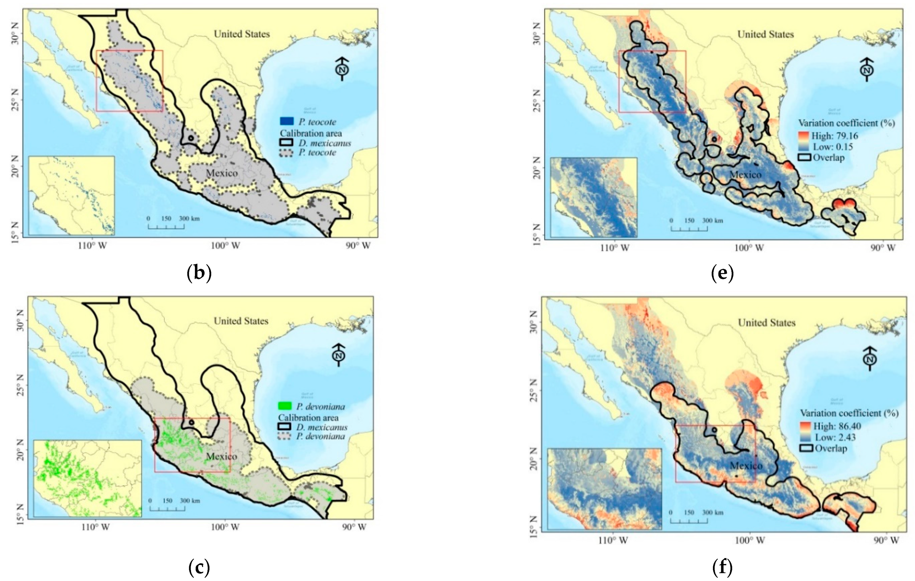
3.6. Overlap of Suitability and Ecological Niches

The overlap of suitable areas of the bark beetle with those of P. leiophylla, P. teocote and P. devoniana in space G is 74.35, 96.98 and 82.44%, respectively (Figure 5a–c). The environmental space (Figure 5d–f) was built with Bio 5, Bio 6, and Bio 12 for the purpose of comparing the fundamental niche and overlap between bark beetle and pine species. In Bio 5 (maximum temperature), the four species have the same tolerances, from 1 to 32 °C (Figure 5d–f); in Bio 6 (minimum temperature) the overlap is −2 to 11 °C, but D. mexicanus has broader tolerance (from −1 to 17 °C). The lowest occurs in P. leiophylla (from −4 to 11 °C). In Bio 12 (annual precipitation), the overlap occurs between 450 and 1755 mm. P. devoniana, the species of limited distribution, possesses the widest interval, from 429 to 2053 mm (Figure 4f); D. mexicanus tolerates a smaller interval (450 to 1755 mm). The fundamental niche of the pine species shows the same disposition in tridimensional space, but different from that of bark beetle species (Figure 5d–f), but in all niches unavailable climate (UC) and the existence of a potential niche (PN) are observed (Figure 5d–f).
Niche similarity between the ‘invasive’ species (D. mexicanus) and the pine species resulted in D = 0.48 and I = 0.67; D = 0.39 and I = 0.61; D = 0.53 and I = 0.69, for P. leiophylla (Figure 6a), P. teocote (Figure 6b) and P. devoniana (Figure 6c). The variance explained by the first two principal components was 61.76% (P. devoniana) to 71.73% (P. leiophylla). In all cases, the variables derived from temperature contributed more in the PCA (PC1) and those of precipitation (PC2) contributed less (Figure 6d–f).
The proportion of the native niche (P. leiophylla, P. teocote and P. devoniana) non–overlapping with the ‘invasive’ niche (D. mexicanus), denoted as Up (Unfilling) is 31.57, 19.44, and 21.15%; niche expansion E is 1.31, 0.84, and 4.62, while niche stability is 98.68, 99.15, and 95.37%, respectively. The shift from niche centroid (C) of the ‘invasive’ species was more significant with P. leiophylla and P. teocote (Figure 6a–b), but in different directions, and almost the same centroid as observed with P. devoniana (Figure 6c). In the three cases, the shift moved over the temperature gradient. Under the similarity hypothesis of ecological niches of the species in niche conservatism (Pinus) and ‘invasive’ species (Dendroctonus), it is observed that both measures of niche similarity are significantly higher than what was expected of this null distribution, with p < 0.05 (Figure 6g–i). Therefore, this hypothesis is rejected, except in the case of D. mexicanus with P. devoniana (Figure 6g–i) where p > 0.05.

4. Discussion

4.1. Species Occurrence Records in ENM

The used of reliable records is fundamental in ENM to avoid bias in prediction, mainly because the primary source of data is an opportunist sampling [22]. In general, 70% of the records were eliminated. The use of altitudinal limits of species distribution in records cleansing has not been documented. Here, it can be observed that altitude (included in the PCA with the Bios) was crucial to identifying atypical and erroneous records of the species, especially within «M». Much has been discussed over the number of species occurrence records to use in ENM; some show that 30 should be a minimum [25], while others indicate that 50 is sufficient [62]. Modeling D. mexicanus in this study was carried out with 86 records. Modeling the pine species surpassed 250 records. Actually, the number of observations is less important than adequately representing species prevalence distributed in the entire geographic and environmental space it occupies [22], for which it is of utmost importance that in SDM and ENM the records comprehend the complete distribution of the species (as was done here). Otherwise, the response of the variables would be wrong [20], as would be the ecological niche. It has been demonstrated that systematic sampling produces greater precision in species distribution models [22]. Some records used here (INFyS) come from this type of sampling, assuring more robust predictions. Moreover, this requirement was corrected by removing spatial autocorrelation.

4.2. Variable Importance in ENM

After Busby (1986) [26] defined bioclimatic variables from precipitation and temperature, a number of different predictors have been generated, but used indistinctly in ENM, despite the fact that some authors [22,29,32] have suggested their use depending on the study scale. Modeling the species of this study was carried out only with bioclimatic variables, [22,29,32]. The rigorous selection of predictors and the best configuration of the algorithm made it possible to choose a robust model to predict the climatic suitability of each species. Other researchers [19] demonstrated that if this process is appropriate the model will show minimum spatial correlation in their residuals. The use of dynamic (bioclimatic) variables for modeling allows determining the vulnerability of a species, in an unstable environment which does not occur with static variables (soil, slope, exposure and altitude) [63]. In 2017, Fourcade and other researchers surprised the scientific community when they demonstrated that pseudo–predictors derived from paints (‘classical paintings’) downloaded from Google Image®, predicted species distribution even better than bioclimatic variables. Undoubtedly, such pseudo–predictors will not satisfy the criteria established in this study (Section 2.2), and so it is crucial to select the environmental predictors in ENM. To generate our models, besides considering these criteria, the ‘kuenm’ algorithm selected the best set of variables based on the validation of 1392 candidate models, using the set of independent records.
It has been demonstrated that using multiple variables brings problems of bias and uncertainty in the predictions [38,42] and a decrease in statistical power; complex models with a large number of parameters tend to overestimate the predictions [38,64] but this depends on the combination of the adjustment parameters of the “regularization multiplier” and “feature classes” [43]. However, this occur especially when the number of records is small [38,64]. Our models included no more than seven predictors avoiding these problems. Other authors argue that a large number of predictors resulted in problems of collinearity [25,35,38], which tend to inflate the variance of response variables and parameters [42], and an erroneous representation of species distribution [16,40], moreover, biological interpretation of the model is complex or null.
Austin (2002) [65] argues that species responses are often nonlinear; likewise, ecological theory suggests response curves are often unimodal [66], and hence, quadratic features may be appropriate. None of our generated models for the studied species was linear; most were quadratic (Table 2), in accord with theory these authors, which demonstrates the correct selection of predictors, quality of records and modeling. Studies reveal that pine species show non–linear responses to climate suitability [67], like what occurs in bark beetle species [18].
Our findings indicate that regardless of the genus and species, the variables of temperature are those that most contributed to the bioclimatic profile, especially seasonal temperature means and extremes (e.g., Bio 10 and Bio 11, Table 3), as occurs in most studies of ENM [67,68,69], even when topographic [28], soil and vegetation [67] variables are included in modeling. For bark beetles, the variables that best predict climatic suitability are temperature [12,70]; e.g., Bio 1 in Dendroctonus rizophagus Thomas & Bright [35]; Bio 5 in Dendroctonus valens Le Conte [71] and Bio 10 in D. mexicanus [18], and in this last species Bio 7, Bio 8, and Bio 10 [28]. It has been found that D. mexicanus possesses a more ample bioclimatic profile than that of several other bark beetle species [18], making it possible to occupy larger geographic areas and probably adapt to new host pine species.
It is surprising that a single variable, e.g., Bio 1 in P. leiophylla and Bio 10 in D. mexicanus, contributes more than 90 and 87%, respectively (Table 3). Like what we found here, it has been demonstrated [71,72] that a single variable predicts plant species distribution very well. In contrast, other authors [23] report models of up to 38 predictors. The number of variables that make up a model (as long as they have been correctly selected) possess a fundamental interpretation. Our analysis shows that this could determine species vulnerability. When the contribution of a single variable is high, there is a risk that if it changes (increases/decreases) and varies over time, it will have important effects on predictions of climate suitability, making the species vulnerable in the same proportions. In contrast, if the model is composed of multiple variables, their contribution would be shared, increasing the possibility that not all are being modified at the same rhythm, even if they do not.
Specifically, in the study area, Bio 1 has increased significantly in recent years [7], a fact that we have verified through climate projections of the GCM’s [33], with an expected increase of 2 to 3.5 °C by the year 2050, making P. leiophylla and D. mexicanus highly vulnerable to climate change. The latter is even more vulnerable because of its high dependence and sensitivity to temperature [10], while P. teocote and P. devoniana are less vulnerable. Previous studies on ecological niche models [42] demonstrate that P. leiophylla is highly vulnerable to climate change, as found here.

4.3. Climate Suitability and Niche Overlap

The stratification of species climate suitability can determine priority areas for conservation or management, especially those of high suitability. The areas of low suitability represent areas that in the past were of medium of high suitability, but nothing can be done to remedy this condition. Low suitability for D. mexicanus (Figure 3a) and P. devoniana (Figure 3d) is observed only at higher latitudes and almost never at lower latitudes, challenging distributional ecology where maximum suitability of the species occurs toward the center of spaces E and G [24]. Analogously, it has been found [13] that greater suitability of D. mexicanus is registered in small portions of the TMVB and the SMOc at higher altitudes and where PinusDendroctonus host diversity is high but discontinuous [14,49]. For Pinus, suitability also occurs at higher altitudes [42], possibly following regimes of higher moisture and lower temperatures.
Superimposing climate suitability (DendroctonusPinus) resulted in very few discontinuous SAP free of SAD (between 30.03 and 25.65%), fortunately, where suitability for pine species is high, in contrast with [49], where less than 1% of all the Pinus host species is D. rhizophagus–free, these differences are explained by the cutoff threshold selected to obtain the overlap. It has been demonstrated that the analysis of suitability overlap in G is problematic because it will depend on the extension and distribution of the environmental gradients in the study area [56]. Despite the importance of identifying SAP–free of SAD, only the study of Smith et al. (2013) [49] is known.
The overlap (D) of the ‘invasive’ species niche with the ‘conservationism’ species with the highest percentage of incidence (P. leiophylla) is almost 50%, but a change in niche of D. mexicanus, relative to the three pine species has been observed (Figure 6a–c). The niche overlap in similar taxonomic groups of pine species is not very high, on average D = 0.20 [67]. Studies reveal that one of the two species (with high plant prevalence) shows a niche shift [20]; this number is quite high, especially in exotic species, it is possible that the studies reported a shift when there was actually none. Less than 1% of the studies show niche conservationism. Some authors [73] suggest that dramatic niche changes found should be carefully interpreted since they are dependent on the methods and data used. The kernel density method in ecological niche studies (used here) is one of the most robust and produces the best results [56,57].

5. Conclusions

Not all the models generated in Maxent were statistically significant (α = 0.05). In ‘kuenm’ it is possible to generate n candidate models and to select a robust model rather than a random model. The statistical procedure (PCA) was a crucial tool for preselecting climate predictors. By including altitude in the analysis (PCA), it was possible to identify atypical and erroneous records within the calibration area, which is not possible through bivariate environmental space. The variables representing extreme temperatures play an important role in defining species climate suitability; they are also indicators of climate change and thus evidence that this will affect species distribution, proportional to their rate of change. The areas of overlapping climate suitability in geographic space and of niches in environmental space average 84.59 and 46.66%, which indicates small areas of Pinus species free of the bark beetle that are isolated in the distribution area. The ordination methods show that pine species have a broader ecological niche, but P. leiophylla and D. mexicanus were identified as highly vulnerable to climate change. In addition, expansion of the bark beetle toward new climates is observed and, consequently, toward new geographic areas following its climate preferences. The areas of high suitability for Pinus, especially those areas free of suitability areas for D. mexicanus, should be prioritized for conservation. The redistribution of the bark beetle species is highly probable in the coming years, consequently, fewer suitable areas for the pine species, free of bark beetle. It is proposed that, when generating ecological niche models, robust methodologies be used, considering the association Dendroctonus–Pinus. This study enriches previous knowledge of the species, improving the delineation of geographic distribution of their ecological niches and specific climate tolerances, contributing tools for the timely implementation of actions and strategies for managing the country’s forests for species conservation and preservation.

Author Contributions

F.M.M.-E. performed analysis of the results and writing original draft preparation of the manuscript. J.M.-G. writing review and editing. R.M.-O., J.Ó.M.L.-D. and J.A.N.-L. assisted in review. All authors have read and agreed to the published version of the manuscript.

Funding

This research was funded by the Forestry National Commission (CONAFOR) and CONACYT, through project number: 2014, C01-234547.

Acknowledgments

To the National Council of Science and Technology (CONACYT) for the scholarship awarded to the first author for postgraduate studies.

Conflicts of Interest

The authors declare no conflict of interest.

Appendix A

Predictive Species Models

Of the thousands of models generated here, it was revealed that not all were statistically significant (10 < n < 99 %), and very few (< 20%) surpassed the omission rate of 5%, demonstrating that using the default parameters in Maxent does not necessarily produce the best model. This has already been demonstrated by several researchers [61,62]. Indeed, some authors indicate that the apparent ‘simplicity’ of Maxent (console Maxent) has caused an exponential increment of modeling studies and that it has only been used as a ‘black box’, while in the ‘kuenm’ software, it is possible to ‘fine tune’ some of the model parameters [43], select sets of variables, and validate the predictive capacity of all the models developed.
Traditionally, the AUC of the ROC has been used as the measure of model fit. However, this statistic has been criticized [47], especially because of its use of back-ground data instead of true absences [46]. Moreover, it is highly sensitive to the study scale, resulting frequently in high AUC values, becoming confused with a good model fit. For this reason, here, we opted for partial ROC, suggested for ENM [46]; we found values between 1.24 (P. leiophylla) and 1.66 (D. mexicanus), where values close to 1 indicate that what was observed coincides with random results, while values above 1 is better than random; that is, model yield is better.

References

  1. del-Val, E.; Sáenz, R.C. Insectos Descortezadores (Coleoptera: Curculionidae) y Cambio Climático: Problemática Actual y Perspectivas En Los Bosques Templados. TIP Rev. Especializada en Cienc. Químico Biol. 2017, 20, 53–60. [Google Scholar] [CrossRef] [Green Version]
  2. Kuennecke, B.H. Temperate Forest Biomes; Greenwood Press: London, UK, 2008; 194p. [Google Scholar]
  3. Challenger, A.; Soberón, J. Los ecosistemas terrestres. In Capital Natural de México; Comisión Nacional para el Conocimiento y Uso de la Biodiversidad: Conabio, México, 2008. [Google Scholar]
  4. Rzedowsky, J. Vegetación de México, 1st ed.; Limusa: México City, México, 1978; p. 432. [Google Scholar]
  5. Gernandt, D.; Pérez-de la Rosa, J. Biodiversidad de Pinophyta (coníferas) en México. Rev. Mex. Biodivers. 2014, 85, 126–133. [Google Scholar] [CrossRef] [Green Version]
  6. Food and Agriculture Organization of the United Nations. El Estado de los Bosques del Mundo. las Vías Forestales Hacia el Desarrollo Sostenible; FAO: Roma, Italy, 2018; p. 52. [Google Scholar]
  7. Allen, M.R.; Dube, O.P.; Solecki, W.; Aragón-Durand, F.; Cramer, W.; Humphreys, S.; Kainuma, M.; Kala, J.; Mahowald, N.; Mulugetta, Y.; et al. Framing and Context. In Global Warming of 1.5 °C. An IPCC Special Report on the Impacts of Global Warming of 1.5 °C above Pre-Industrial Levels and Related Global Greenhouse Gas Emission Pathways, in the Context of Strengthening the Global Response to the Threat of Climate Change, Sustainable Development, and Efforts to Eradicate Poverty; Masson-Delmotte, V., Zhai, V., Portner, H., Roberts, D., Skea, J., Shukla, P., Pirani, A., Moufouma-Okia, W., Chen, Y., Zhou, X., et al., Eds.; IPCC: Geneve, Switzerland, 2018. [Google Scholar]
  8. Wood, S.L. The Bark and Ambrosia Beetles of North and Central America (Coleoptera: Scolytidae) a Taxonomic Monograph; Great Basin Naturalist Memoirs: Provo, UT, USA, 1982; p. 1359. [Google Scholar]
  9. Armendáriz, T.F.; Torres, B.V.; Fernanda, L.M.; Villa, C.J.; Zúñiga, G. New record and extension of the distribution range of the bark beetle Dendroctonus rhizophagus (Curculionidae: Scolytinae). Rev. Mex. Biodivers. 2012, 83, 850–853. [Google Scholar] [CrossRef]
  10. Bentz, B.J.; Jönsson, A.M. Modeling bark beetle responses to climate change. In Bark Beetles: Biology and Ecology of Native and Invasive Species; Vega, F.E., Hofstetter, R.W., Eds.; Academic Press: London, UK, 2015; pp. 533–553. [Google Scholar]
  11. Six, D.; Bracewell, R. Dendroctonus. In Bark Beetles: Biology and Ecology of Native and Invasive Species; Vega, F.E., Hofstetter, R.W., Eds.; Academic Press: London, UK, 2015; pp. 305–350. [Google Scholar]
  12. Bentz, B.; Régnière, J.; Fettig, C.; Hansen, E.M.; Hayes, J.L.; Hicke, J.A.; Kelsey, R.J.; Negrón, J.F.; Seybold, S.J. Climate change and bark beetles of the western United States and Canada: Direct and indirect effects. BioScience 2010, 60, 602–613. [Google Scholar] [CrossRef]
  13. Salinas, M.Y.; Ager, A.; Vargas, C.F.; Hayes, J.L.; Zúñiga, G. Determining the vulnerability of Mexican pine forests to bark beetles of the genus Dendroctonus Erichson (Coleoptera: Curculionidae: Scolytinae). For. Ecol. Manag. 2010, 260, 52–61. [Google Scholar] [CrossRef]
  14. Salinas, M.Y.; Mendoza, G.M.; Barrios, M.A.; Cisneros, R.; Macías, S.J.; Zúñiga, G. Areography of the genus Dendroctonus (Coleoptera: Cur-culionidae: Scolytinae) in México. J. Biogeogr. 2004, 31, 1163–1177. [Google Scholar] [CrossRef]
  15. Cibrián, T.D.; Méndez, M.J.; Campos, B.R.; Yates, H.O.; Flores, L.J. Insectos Forestales de México; Universidad Autónoma de Chapingo: Estado de México, México, 1995; p. 453. [Google Scholar]
  16. Peterson, A.T.; Soberón, J.; Pearson, R.G.; Anderson, R.P.; Martínez, M.E.; Nakamura, M.; Araújo, M.B. Ecological Niches and Geographic Distributions; Princeton University Press: Pricenton, NJ, USA, 2011. [Google Scholar]
  17. Cobos, M.E.; Jiménez, L.; Nuñez, P.C.; Romero, A.D.; Simões, M. Sample data and training modules for cleaning biodiversity information. Biodivers. Inform. 2018, 14, 49–50. [Google Scholar] [CrossRef] [Green Version]
  18. Méndez, E.F.; Méndez, G.J.; Cerano, P.J. Distribución actual y potencial de Dendroctonus mexicanus Hopkins bajo dos escenarios de cambio climático. Madera Y Bosques 2020, 26, 1–14. [Google Scholar] [CrossRef]
  19. Elith, J.; Leathwick, J. Species distribution models: Ecological explanation and prediction across space and time. Annu. Rev. Ecol. Evol. Syst. 2009, 40, 677–697. [Google Scholar] [CrossRef]
  20. Guisan, A.; Petitpierre, B.; Broennimann, O.; Daehler, C.; Kueffer, C. Unifying niche shift studies: Insights from biological invasions. Trends Ecol. Evol. 2014, 29, 260–269. [Google Scholar] [CrossRef] [Green Version]
  21. Soberón, J.; Osorio, O.L.; Peterson, A.T. Diferencias conceptuales entre modelación de nichos y modelación de áreas de distribución. Rev. Mex. Biodivers. 2017, 88, 437–441. [Google Scholar] [CrossRef]
  22. Franklin, J. Mapping Species Distributions: Spatial Inference and Prediction; Cambridge University Press: Cambridge, UK, 2009. [Google Scholar]
  23. Austin, M.P.; Van Niel, K.P. Improving species distribution models for climate change studies: Variable selection and scale. J. Biogeogr. 2011, 38, 1–8. [Google Scholar] [CrossRef]
  24. Guisan, A.; Zimmermann, N.E. Predictive habitat distribution models in ecology. Ecol. Model. 2000, 135, 147–186. [Google Scholar] [CrossRef]
  25. Elith, J.; Graham, C.H.; Anderson, R.P.; Dudík, M.; Ferrier, S.; Guisan, A.; Hijmans, R.J.; Huettmann, F.; Leathwick, J.R.; Lehmann, A.; et al. Novel methods improve prediction of species’ distributions from occurrence data. Ecography 2006, 29, 129–151. [Google Scholar] [CrossRef] [Green Version]
  26. Busby, J.R. A biogeoclimatic analysis of Nothofagus cunninghamii (Hook.) Oerst. In southeastern Australia. Aust. Ecol. 1986, 11, 1–7. [Google Scholar] [CrossRef]
  27. Fourcade, Y.; Besnard, A.G.; Secondi, J. Paintings predict the distribution of species, or the challenge of selecting environmental predictors and evaluation statistics. Glob. Ecol. Biogeogr. 2018, 27, 245–256. [Google Scholar] [CrossRef]
  28. González, H.A.; Morales, V.R.; Romero, S.M.; Islas, T.B.; Pérez, M.R. Modelling potential distribution of a pine bark beetle in Mexican temperate forests using forecast data and spatial analysis tools. J. For. Res. 2020, 31, 649–659. [Google Scholar] [CrossRef]
  29. Soberón, J.; Peterson, T.A. Interpretation of models of fundamental ecological niches and species’ distributional areas. Biodivers. Inform. 2005, 2, 1–10. [Google Scholar] [CrossRef] [Green Version]
  30. Hutchinson, G.E. Concluding remarks. Cold Spring Harbor on Quantitative Symposia Biology. GS Search 1957, 22, 415–427. [Google Scholar]
  31. Warren, D.L.; Glor, R.E.; Turelli, M. Environmental niche equivalency versus conservatism: Quantitative approaches to niche evolution. Evolution 2008, 62, 2868–2883. [Google Scholar] [CrossRef] [PubMed]
  32. Willis, K.J.; Whittaker, R.J. Species diversity-scale matters. Science 2002, 295, 1245–1248. [Google Scholar] [CrossRef] [PubMed]
  33. Karger, D.N.; Conrad, O.; Böhner, J.; Kawohl, T.; Kreft, H.; Soria, A.R.; Zimmermann, N.E.; Linder, H.P.; Kessler, M. Climatologies at high resolution for the earth’s land surface areas. Sci. Data 2017, 4, 1–20. [Google Scholar] [CrossRef] [Green Version]
  34. Escobar, L.E.; Lira, N.A.; Medina, V.G.; Peterson, A.T. Potential for spread of the white-nose fungus (Pseudogymnoascus destructans) in the Americas: Use of Maxent and NicheA to assure strict model transference. Geospat. Health 2014, 9, 221–229. [Google Scholar] [CrossRef]
  35. Mendoza, M.G.; Salinas, M.Y.; Olivo, M.A.; Zúñiga, G. Factors influencing the geographical distribution of Dendroctonus rhizophagus (Coleoptera: Curculionidae: Scolytinae) in the Sierra Madre Occidental, Mexico. Environ. Entomol. 2011, 40, 549–559. [Google Scholar] [CrossRef] [PubMed] [Green Version]
  36. Lê, S.; Josse, J.; Husson, F. FactoMineR: An R Package for multivariate analysis. J. Stat. Softw. 2008, 25, 1–18. [Google Scholar] [CrossRef] [Green Version]
  37. Merow, C.; Smith, M.J.; Silander, J.A. A practical guide to MaxEnt for modeling species’ distributions: What it does, and why inputs and settings matter. Ecography 2013, 36, 1058–1069. [Google Scholar] [CrossRef]
  38. De Marco, P.; Nóbrega, C.C. Evaluating collinearity effects on species distribution models: An approach based on virtual species simulation. PLoS ONE 2018, 13, e0202403. [Google Scholar] [CrossRef]
  39. Sturges, H.A. The choice of a class interval. J. Am. Stat. Assoc. 1926, 21, 65–66. [Google Scholar] [CrossRef]
  40. Beaumont, L.J.; Hughes, L.; Poulsen, M. Predicting species distributions: Use of climatic parameters in BIOCLIM and its impact on predictions of species’ current and future distributions. Ecol. Model. 2005, 186, 251–270. [Google Scholar] [CrossRef]
  41. Aiello-Lammens, M.E.; Boria, R.A.; Radosavljevic, A.; Vilela, B.; Anderson, R.P. spThin: An R package for spatial thinning of species occurrence records for use in ecological niche models. Ecography 2015, 38, 541–545. [Google Scholar] [CrossRef]
  42. Cruz, C.G.; López, M.L.; Villaseñor, J.L.; Ortiz, E. Potential species distribution modeling and the use of principal component analysis as predictor variables. Rev. Mex. Biodivers. 2014, 85, 189–199. [Google Scholar] [CrossRef]
  43. Cobos, M.E.; Peterson, A.T.; Barve, N.; Osorio, O.L. kuenm: An R package for detailed development of ecological niche models using Maxent. PeerJ 2019, 7, e6281. [Google Scholar] [CrossRef] [PubMed] [Green Version]
  44. Elith, J.; Kearney, M.; Phillips, S. The art of modelling range-shifting species. Methods Ecol. Evol. 2010, 1, 330–342. [Google Scholar] [CrossRef]
  45. Phillips, S.J.; Dudik, M. Modeling of species distributions with MaxEnt: New extensions and a comprehensive evaluation. Ecography 2008, 31, 161–175. [Google Scholar] [CrossRef]
  46. Phillips, S.J.; Anderson, R.P.; Schapire, R.E. Maximum entropy modeling of species geographic distributions. Ecol. Model. 2006, 190, 231–259. [Google Scholar] [CrossRef] [Green Version]
  47. Peterson, A.T.; Papeş, M.; Soberón, J. Rethinking receiver operating characteristic analysis applications in ecological niche modeling. Ecol. Model. 2008, 213, 63–72. [Google Scholar] [CrossRef]
  48. Morales, N.S.; Fernández, I.C.; Baca-González, V. MaxEnt’s parameter configuration and small samples: Are we paying attention to recommendations? A systematic review. PeerJ 2017, 5, e3093. [Google Scholar] [CrossRef]
  49. Smith, S.E.; Mendoza, M.G.; Zúñiga, G.; Halbrook, K.; Hayes, J.L.; Byrne, D.N. Predicting the distribution of a novel bark beetle and its pine hosts under future climate conditions. Agric. For. Entomol. 2013, 15, 212–226. [Google Scholar] [CrossRef]
  50. Lobo, J.M.; Jimenez, V.A.; Real, R. AUC: A misleading measure of the performance of predictive distribution models. Glob. Ecol. Biogeogr. 2007, 17, 145–151. [Google Scholar] [CrossRef]
  51. Reddy, K.G.; Khan, M.G. stratify: An R Package for optimal stratification and sample allocation for univariate populations. Aust. N. Z. J. Stat. 2020, 62, 383–405. [Google Scholar] [CrossRef]
  52. Khan, E.A.; Khan, M.M.; Ahsan, M.J. Optimum stratification: A mathematical programming approach. Calcutta Stat. Assoc. Bull. 2002, 52, 323–333. [Google Scholar] [CrossRef]
  53. Khan, M.M.; Nand, N.; Ahmad, N. Determining the optimum strata boundary points using dynamic programming. Surv. Methodol. 2008, 34, 205–214. [Google Scholar]
  54. Khan, M.M.; Reddy, K.G.; Rao, D.K. Designing stratified sampling in economic and business surveys. J. Appl. Stat. 2015, 42, 2080–2099. [Google Scholar] [CrossRef]
  55. Schoener, T.W. Nonsynchronous spatial overlap of lizards in patchy habitats. Ecology 1970, 51, 408–418. [Google Scholar] [CrossRef] [Green Version]
  56. Broennimann, O.; Fitzpatrick, M.C.; Pearman, P.B.; Petitpierre, B.; Pellissier, L.; Yoccoz, N.G.; Thuiller, W.; Fortin, M.J.; Randin, C.; Zimmermann, N.E.; et al. Measuring ecological niche overlap from occurrence and spatial environmental data. Glob. Ecol. Biogeogr. 2012, 221, 481–497. [Google Scholar] [CrossRef] [Green Version]
  57. Godsoe, W.; Case, B.S. Accounting for shifts in the frequency of suitable environments when testing for niche overlap. Methods Ecol. Evol. 2015, 6, 59–66. [Google Scholar] [CrossRef]
  58. Sánchez, G.A. Una visión actual de la diversidad y distribución de los pinos de México. Madera Y Bosques 2008, 14, 107–120. [Google Scholar] [CrossRef] [Green Version]
  59. Di Cola, V.; Broennimann, O.; Petitpierre, B.; Breiner, F.T.; D’Amen, M.; Randin, C.; Engler, R.; Pottier, J.; Pio, D.; Dubuis, A.; et al. ecospat: An R package to support spatial analyses and modeling of species niches and distributions. Ecography 2016, 40, 774–787. [Google Scholar] [CrossRef]
  60. R Core Team. R: A Language and Environment for Statistical Computing; Foundation for Statistical Computing: Vienna, Austria, 2020; Available online: https://www.r-project.org/ (accessed on 11 May 2020).
  61. Loiselle, B.A.; Jørgensen, P.M.; Consiglio, T.; Jiménez, I.; Blake, J.G.; Lohmann, L.G.; Montiel, O.M. Predicting species distributions from herbarium collections: Does climate bias in collection sampling influence model outcomes. J. Biogeogr. 2008, 35, 105–116. [Google Scholar] [CrossRef]
  62. Shcheglovitova, M.; Anderson, R.P. Estimating optimal complexity for ecological niche models: A jackknife approach for species with small sample sizes. Ecol. Model. 2013, 269, 9–17. [Google Scholar] [CrossRef]
  63. Radosavljevic, A.; Anderson, R.P. Making better Maxent models of species distributions: Complexity, overfitting and evaluation. J. Biogeogr. 2014, 41, 629–643. [Google Scholar] [CrossRef]
  64. Phillips, S.J.; Dudík, M.; Schapire, R.E. A maximum entropy approach to species distribution modeling. In Proceedings of the Twenty-First International Conference on Machine Learning—ICML, Banff, AB, Canada, 4–8 July 2004. [Google Scholar]
  65. Austin, M. Spatial prediction of species distribution: An interface between ecological theory and statistical modelling. Ecol. Model. 2002, 157, 101–118. [Google Scholar] [CrossRef] [Green Version]
  66. Austin, M. Species distribution models and ecological theory: A critical assessment and some possible new approaches. Ecol. Model. 2007, 200, 1–19. [Google Scholar] [CrossRef]
  67. Aguirre, G.J.; Serna, C.H.; Villalobos, A.A.; Pérez, D.J.; Raes, N. Similar but not equivalent: Ecological niche comparison across closely–related Mexican white pines. Divers. Distrib. 2015, 21, 245–257. [Google Scholar] [CrossRef]
  68. Williams, D.W.; Liebhold, A.M. Climate change and the outbreak ranges of two North American bark beetles. Agric. For. Entomol. 2002, 4, 87–99. [Google Scholar] [CrossRef]
  69. Stockwell, D. Improving ecological niche models by data mining large environmental datasets for surrogate models. Ecol. Model. 2006, 192, 188–196. [Google Scholar] [CrossRef] [Green Version]
  70. Pureswaran, D.S.; Roques, A.; Battisti, A. Forest insects and climate change. Curr. For. Rep. 2018, 4, 35–50. [Google Scholar] [CrossRef] [Green Version]
  71. Maldonado, M.J.; Cera, J.I.; Mendoza, A.R.; Sáenz, L.A.; Torres, O.M.; Bravo, P.L.; Alatorre, C.L. Distribución potencial de Dendroctonus valens mediante modelos de máxima entropía: Estado de California, E.U. Rev. Latinoam. El Ambiente Y Las Cienc. 2015, 6, 194–198. [Google Scholar]
  72. Pearman, P.B.; Randin, C.F.; Broennimann, O.; Vittoz, P.; Knaap, W.O.; Engler, R.; Le-Lay, G.; Zimmermann, N.; Guisan, A. Prediction of plant species distributions across six millennia. Ecol. Lett. 2008, 11, 357–369. [Google Scholar] [CrossRef]
  73. Broennimann, O.; Treier, U.A.; Müller-Schärer, H.; Thuiller, W.; Peterson, A.T.; Guisan, A. Evidence of climatic niche shift during biological invasion. Ecol. Lett. 2007, 10, 701–709. [Google Scholar] [CrossRef] [Green Version]
Figure 1. Study area that includes temperate forests.
Forests 12 00385 g001
Figure 2. General scheme of steps and procedures for ecological niche model generation.
Forests 12 00385 g002
Figure 3. Climate suitability for: (a) Dendroctonus mexicanus, (b) Pinus leiophylla, (c) Pinus teocote, and (d) Pinus devoniana, stratified in medium, high and low, according to the minimum and maximum intra-stratum variance among them, solved by using a dynamic programming technique.
Forests 12 00385 g003
Figure 4. Suitable areas free of the bark beetle for: (a) Pinus leiophylla (orange color), (b) Pinus teocote (blue color), and (c) Pinus devoniana (green color), suitable areas free of the bark beetle Dendroctonus mexicanus. Average uncertainty, expressed as variation coefficient of the prediction model of each pine species (df), respectively. The continuous line is the bark beetle calibration area; dotted line and shaded area is the pine species calibration area.
Forests 12 00385 g004aForests 12 00385 g004b
Figure 5. Overlap of climate suitability of Dendroctonus mexicanus with Pinus leiophylla. (a), Pinus teocote (b) and Pinus devoniana (c) in the geographic space. Overlap of niches in the environmental space of this same species association (df), composed of three bioclimatic dimensions (Bio 5: Max Temperature of Warmest Month in °C ×10), Bio 6: Min Temperature of Coldest Month in °C ×10 and Bio 12: Annual Precipitation in mm). Each blue dot corresponds to the environmental combination represented in one of 50,000 grid cells at 5 × 5 km of spatial resolution, unavailable climate (UC) and potential niche (PN).
Forests 12 00385 g005
Figure 6. Niche of the species along the two first axes of the PCA (ac) of the native species and ‘invasive’ species. Green (Pinus) and blue (Dendroctonus mexicanus) (D), shading shows the density of the occurrences of the species by cell. The solid and dashed contour lines illustrate, respectively, 100% and 95% of the available (background) environment, E represents niche expansion and Up the non-overlapping niche between pine species and the ‘invasive’ species. The arrows represent the change of the niche centroid of the ‘invasive’ species, relative to the ‘native’ species. The contribution of the climatic variables on the two axes of the PCA and the percentage of inertia explained by the two axes (df). Histograms show the observed niche similarity I between the two ranges (lines with a diamond) and simulated niche similarity (grey bars). Pinus leiophylla (a,d,g), Pinus teocote (b,e,h) and Pinus devoniana (c,f,i).
Forests 12 00385 g006
Table 1. Contribution of the bioclimatic variables determined by principal component analysis for their preselection and accommodation in different sets to conduct the species climate suitability modeling tests.
Variable NameDescriptionSpecies
Dendroctonus mexicanusPinus leiophyllaPinus teocotePinus devoniana
PC1 (48.7)PC2 (18.9)PC1 (43.9)PC2 (29.5)PC1 (39.6)PC2 (26.0)PC1 (35.0)PC2 (29.1)
Bio 1Annual Mean Temperature (°C)11.44 (3) 14.61 (3) 15.1315.75 (3)
Bio 2Annual Mean Diurnal Range (°C) 3.9711.24 (1,2,3) 13.50 8.19
Bio 3Isothermality (%)7.04 (1) 13.20 (2) 7.70 3.35
Bio 4Temperature Seasonality (%)9.99 14.23 13.41 (1,2,3) 7.68 (1,2,3)
Bio 5Max Temperature of Warmest Month (°C) 9.08 7.58 (1) 13.31 12.28
Bio 6Min Temperature of Coldest Month (°C)14.87 (2) 9.82 (2) 12.36 (1,2,3) 20.08 (2)
Bio 7Annual Temperature Range (°C) 8.1814.33 (1,3) 14.86 (1,2,3) 9.24 (1,2,3)
Bio 10Mean Temperature of Warmest Quarter (°C) 9.85 (1,2,3) 9.83 (2) 14.42 (1,2)11.40
Bio 11Mean Temperature of Coldest Quarter (°C)16.43 (1) 9.36 (1) 10.31 (1,2,3) 18.83 (1)
Bio 12Annual Precipitation (mm) 17.59 9.01 (1,2,3)7.62 (1,2,3) 13.59 (1,2,3)
Bio 13Precipitation of Wettest Month (mm) 14.70 7.484.00 5.88
Bio 14Precipitation of Driest Month (mm)6.00 12.70 10.54 10.43
Bio 15Precipitation Seasonality (CV, %)9.15 (1,3) 4.53 (1) 4.43 (1) 4.56
Bio 16Precipitation of Wettest Quarter (mm) 15.04 (1,2,3) 6.56 3.54 5.99
Bio 17Precipitation of Driest Quarter (mm)6.68 13.88 11.10 10.80
Note: PC = principal component; in parentheses, the variance explained is indicated in %, (1,2,3) = set number, indicating the reaccomodation of the bioclimatic variable in the corresponding set. = values × 10.
Table 2. Candidate models generated and selected, and their fit and validation statistics.
Criterion/SpeciesD. mexicanusP. leiophyllaP. teocoteP. devoniana
Calibration and evaluation of candidate models
TCM1392139213921392
SSM13837451328132
MCOr2620763201
MAIC1312
n of SSM and MCOr2540763201
n of SSM and MAIC1312
n of SSM, MCOr and MAIC1011
Selected modelM_2_F_t (2)M_5_q (3)M_3_F_qth (1)M_2_F_qh (1)
Statistics of the selected model
Mean AUC ratio1.661.241.491.35
Rate of omission > 0.05%0.050.770.040.03
AICc1683.3417393.4213851.284900.27
delta AICc21.6252.84251.3561.26
TCM = total candidate models; SSM = statistically significant models; MCOr = models that satisfy the criterion of omission rate, MAIC = models that satisfy the AICc; AICc = Aikaike information criterion, (1,2,3) = set number.
Table 3. Relative contribution (in percentage) of the suitability model bioclimatic variables of each species determined by the jackknife test and the detailed bioclimatic profile of the species.
VariableContrib.Dendroctonus mexicanus
Name(%)LengthMeanMeanCI0.050.100.25Median0.750.900.95RangeSDCVMADIQR
Bio 64.78653.0±7.0−10.16.734.055.274.395.6100.6153.832.561.331.440.3
Bio 1087.886180.7±5.6140.5149.6166.3178.7201.3218.5221.2130.726.114.428.135.0
Bio 153.28689.2±2.765.971.879.890.7100.2103.4106.452.612.614.114.320.4
Bio 164.386578.2±43.7307.8325.0430.5546.0708.8877.0962.0834.0204.035.3201.6278.3
Pinus leiophylla
Bio 193.9900138.7±1.2111.9116.1126.5136.4149.5164.1171.499.017.912.917.123.0
Bio 25.6900118.9±0.795.1103.1116.8123.0125.7128.1129.062.311.09.34.99.0
Bio 70.5900246.6±2.8169.3181.2219.9253.9277.4297.1305.8202.242.117.140.557.5
Pinus teocote
Bio 43.87353363.6±79.61195.51553.32962.33628.83956.44698.74916.2533.61098.532.7600.7994.1
Bio 615.673518.4±2.7−19.5−14.6−6.43.537.078.193.9195.536.6198.920.143.4
Bio 73.3735227.9±2.8156.2164.3212.2238.3251.5269.1275.3200.038.016.723.139.3
Bio 1063.8735178.5±1.3152.6158.2166.7176.0187.9201.9210.9150.318.510.414.921.1
Bio 11573587.6±2.351.857.366.176.9102.8138.5153.6183.431.836.320.636.6
Bio 126.5735901.0±18.0581.7626.0723.0847.01045.51250.61392.91424.0248.527.6225.4322.5
Bio 152.173592.1±0.971.476.583.992.9101.1106.5110.376.011.812.812.917.2
Pinus devoniana
Bio 428.22551813.2±61.31072.31165.81523.71780.21985.42440.02745.92892.5497.327.4338.6461.7
Bio 71.3255181.9±3.2132.0139.0162.7189.6199.1212.2218.3115.326.114.323.436.4
Bio 1150.8255141.9±3.599.8107.2119.3139.7162.0176.8188.3140.527.519.431.742.7
Bio 1219.82551090.0±40.5608.8712.4858.51043.01265.51579.41770.81624.0328.730.2309.9407.0
MeanCI = confidence interval of mean, 0.05, 0.95 = quantiles of the bioclimatic variable, SD = standard deviation, CV = coefficient of variation (%); MAD = median absolute deviation, IQR = interquartile range.
Publisher’s Note: MDPI stays neutral with regard to jurisdictional claims in published maps and institutional affiliations.

