

Spatiotemporal Variability in Disturbance Frequency and Severity across Mexico: Evidence from Conifer Tree Rings
by
 ,
,
Marín Pompa-García
1,* ,
,
Jan Altman
2,3,
Daniela Sarahi Paéz-Meráz
1 and
José Alexis Martínez Rivas
1
1
Laboratorio de Dendroecología, Facultad de Ciencias Forestales, Universidad Juárez del Estado de Durango, Río Papaloapan y Blvd. Durango S/N Col. Valle del Sur, Durango 34120, Mexico
2
Czech Academy of Sciences, Institute of Botany, Dukelská 135, 379 01 Třeboň, Czech Republic
3
Faculty of Forestry and Wood Sciences, Czech University of Life Sciences Prague, Kamýcká 129, 165 00 Praha-Suchdol, Czech Republic
*
Author to whom correspondence should be addressed.
Forests 2023, 14(5), 900; https://doi.org/10.3390/f14050900
Submission received: 26 November 2022
/
Revised: 9 January 2023
/
Accepted: 25 April 2023
/
Published: 27 April 2023
(This article belongs to the Section Forest Inventory, Modeling and Remote Sensing)
Abstract
:It is critical to understand the ecological processes of forest dynamics by identifying past forest disturbances to take appropriate management actions. Tree-rings are commonly used for this purpose due to their reliability and accuracy. Here, we used a network of ring-width data distributed along a broad ecological gradient for the spatiotemporal identification of forest disturbances in 15 species of 13 sites of young Mexican conifers. We found different spatial and temporal patterns in the occurrence of forest disturbance. The species with the highest disturbance rates were Pinus patula (Ppa; El Jacalón), Pinus montezumae (Pmo; La Cueva), Pinus hartwegii (Phc; Cerro El Moro), and Pinus teocote (Pts; Rancho Joyas del Durazno) of the Gulf of Mexico, and Pinus ayacahuite (Pay; Corral de los Borregos) of the Mexico Center. The highest number of disturbances was found in 1953, 1956, 1976, and 1980; however, we noted that the number of disturbances tended to increase from 1975 to 1990 and particularly from 2000 onwards. The species close to the Gulf of Mexico presented a higher frequency and severity of disturbances than those located close to the Pacific Ocean. Thus, our results demonstrate a spatiotemporal pattern of disturbance events, which deserves further analysis, including regarding the drivers of disturbance. This knowledge is crucial for a better understanding of the dynamics of contemporary species.
1. Introduction
Understanding forest ecosystem dynamics has essential implications for the demands of sustainable forest management in the face of climate change scenarios [1].
It is recognized that forest ecosystems undergo constant change due to disturbances, but also because of the direct and indirect effects of changing temperatures and CO2 emissions [2,3]. Such disturbance regimes lead to changes in the forest structure and composition, especially the transformation of old stands into young stands [4]. Understanding the role of temporal and spatial disturbances can provide critical insights into the biogeography of forests [5]. Forest ecology research must therefore focus on accurate spatial and temporal information regarding past forest disturbances [6]. In this regard, the retrospective study of releases (i.e., abrupt and sustained increases in radial tree growth) using tree-ring analysis is a widely used approach to reconstruct historical forest disturbances [7,8]. The tree-ring approach provides a robust estimate of past disturbance events [9].
Tree-rings have been used worldwide for the growth release analysis and reconstruction of historical disturbance [10], disturbance dynamics [11], the identification of disturbance agents and temporal and spatial differences in disturbance severity, and the proportion of the stand disturbed [12], comparisons of disturbance reconstruction among radial increment cores [13], tree canopy disturbance in order to refine dendroclimatic reconstructions [14], and the integration of paleo-ecological approaches [15], etc.
Globally, most tree-ring-based disturbance reconstructions have been conducted in Europe and North America [16], while few studies are available for other parts of the world, including Mexico [17]. In this country, despite the tree diversity found in various ecological niches, there have been only limited applications of dendroecology in the study of disturbances such as hurricane damage [18] or fires [19], or with BAI modelling used as a proxy for disturbances [20]. Consequently, the study of disturbance must be improved, using a spatiotemporal perspective as an ideal strategy to improve the scientific knowledge of forest dynamics in these ecosystems. These forests are characterized by diverse and mostly young conifers, and represent the current structure [21], and their analysis is gaining importance given their high productivity [22]. The region is home to a great diversity of taxa, comprising 10 genera including Pinus, Abies, and Juniperus, with a high degree of endemism [23].
Using a network of ring datasets distributed along a broad ecological gradient, we identified disturbances and analyzed the spatial and temporality variability of past disturbances along geographical gradients in contemporary Mexican conifer forests. We hypothesized that a network of tree-ring datasets will identify spatial and temporal patterns in disturbance events across contemporary Mexican coniferous forests.
This cross-species approach is expected to increase knowledge of the spatiotemporal patterns of forest disturbances in contemporary Mexican conifer forests for subsequent research.
2. Materials and Methods
2.1. Study Area
Thirteen species were selected that occur along a bioclimatic gradient of Mexico, which is characterized as a highly diverse region of the planet [24] (Table 1). The gradient ranged in elevation from 713 to 3500 m asl. All of the sites corresponded to young and unevenly aged forest stands in which the predominant species in each site comprised at least 70% of its basal area.
At each site, a central tree was randomly selected for each species, and a further nineteen of the closest individual trees were then sampled. From these, at least two radial cores were taken using a Pressler increment borer (Ø = 5 mm) at a height of 1.3 m above ground level, a standard known in forestry as diameter at breast height (DBH, cm).
2.2. Ring Width Data
Radial increment cores were mounted on wooden racks and polished with increasingly fine sandpaper. Tree-ring width (TRW) was measured using a VELMEX ultra-precision (0.01 mm) measuring system. Cross-dating of samples from the same species and location was performed. Visual dating was verified by statistical validation using the program COFECHA [25], which compares the ring series of each individual tree with a master chronology for each species. We built species tree-ring width chronologies using standard dendrochronological procedures [25]. We calculated the mean values of inter-tree correlation (Rbt), subsample signal strength (SSS), and expressed population signal (EPS), where a minimum threshold of 0.85 is normally considered indicative of well-replicated chronologies [26] (see Table A1; Figure A1 in Appendix A).
2.3. Disturbance Identification
The boundary line method proposed by Black and Abrams [27] was used to identify disturbances. This methodology included prior growth, in which releases within 20%–49.9% and 50%–100% of the limit line were considered. The effect of prior growth on the release response was evaluated by plotting prior growth against percentage change in growth. The percent change in growth was calculated using the following formula (Equation (1)):
where:
M1 = average growth over the previous 10 years;
M2 = average growth over the next 10 years.
Prior growth was defined as the average gross growth in the 10 years preceding each annual ring. Prior growth and percentage change in growth were both calculated for each year of each series using the RWL files.
The TRADER package [28] was used to determine the frequency and intensity of disturbances using R software [29]. We analyzed only the common period from 1950 to 2010, and all detected releases above a 20% threshold were considered disturbance events according to the suggested threshold by the original methodology [27]. We did not divide releases into categories as we are interested in the general pattern, and we could not connect these with the recorded severity of disturbances as these are not known [6]. Detected releases were grouped into 5-year intervals. This strategy was based on our previous knowledge of the territory and experience in dendrosciences [17].
2.4. Spatial Characterization of Disturbances
For spatial characterization of disturbances, growth releases were identified according to their vicinity with respect to the Gulf of Mexico, Mexico Center, and the Pacific Ocean. In addition, kernel density estimation (KDE) was used for two different time periods: 1950–1980 and 1981–2010. This is a nonparametric statistical method for estimating spatial density that has been used previously in Mexico for predicting forest disturbances, especially wildfires, e.g., [30]. Although disturbances drivers were beyond the scope of our study, we complementarily explored drought as a potential factor in the spatial variation in disturbance distribution. We calculated the Standardized Precipitation Evapotranspiration Index (SPEI) (see https://spei.csic.es/map/maps.html#months=7#month=8#year=2021, accessed on 23 May 2022). This multi-scalar drought index is an ideal strategy to address geographic disturbances–hydroclimatic relationships, given that it utilizes data pertaining to spatio-temporally accumulated droughts. This evidences a close correlation between evaporative demand and its influence on growth fluctuations. Thus, negative values signify a water deficit, indicating drought, and vice versa. We obtained SPEI data at a 0.5° spatial resolution from the SPEI Global Drought Monitor webpage (https://spei.csic.es/map/maps.html, accessed on 30 May 2022).
3. Results
3.1. Identification of Temporal Disturbances
Disturbances were recorded for at least one species in 36 of the 60 years analyzed during the common period from 1950 to 2010 (Figure 1).
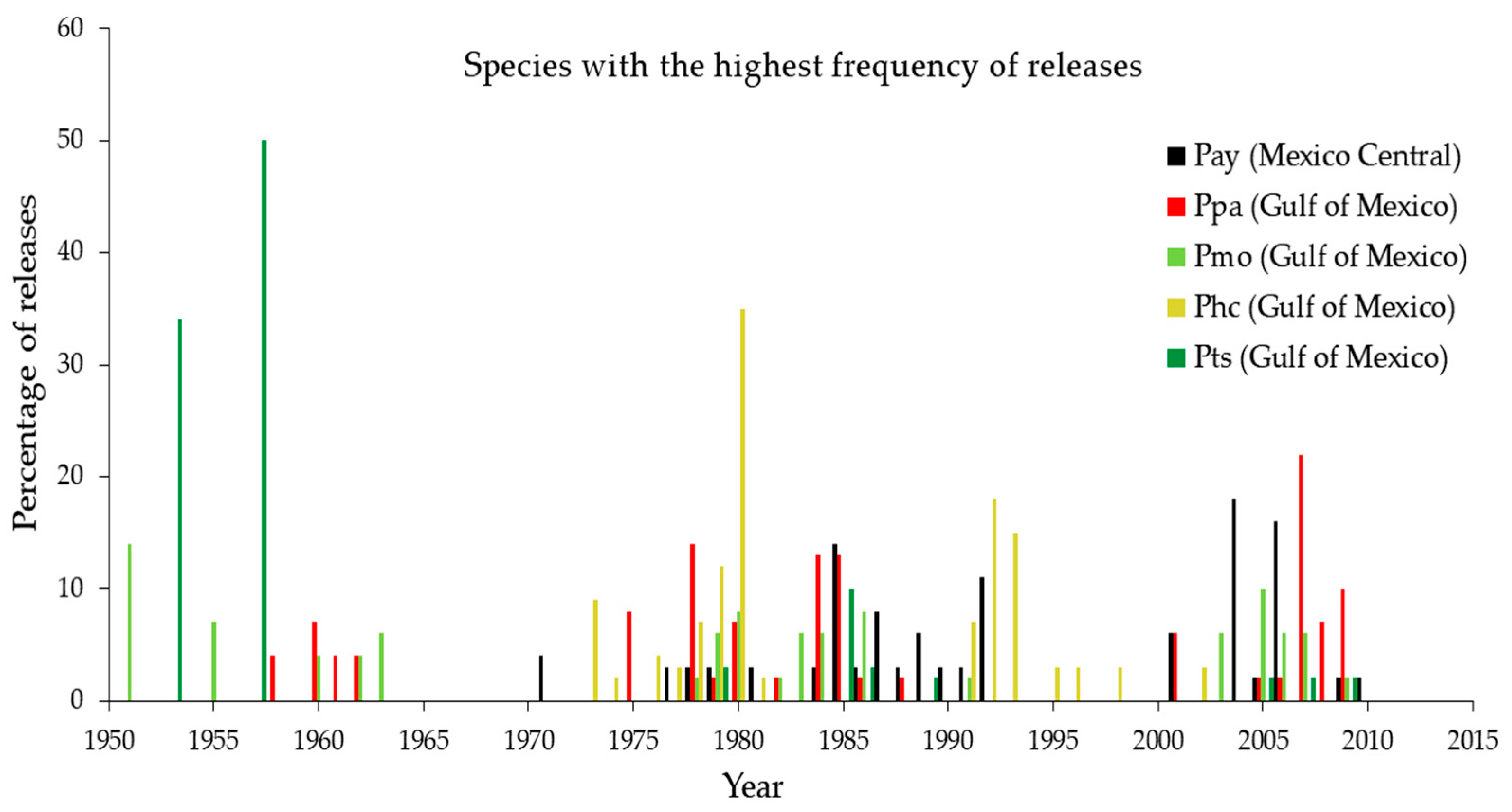
The periods with the highest number of disturbances per species (Pay, Ppa, Pmo, Phc, and Ptn) were 1953, 1956, 1976, and 1980. In general, a higher occurrence of disturbances was observed from 2000 onward (Figure 2). The species with the highest number of disturbances neighboring the Pacific Ocean was Pce during 1967, 1978, and 2009. At the easterm sites close to the Gulf of Mexico, Ptn, Pmo, Ppa, Phc, and Pse presented the highest percentage of cores with disturbances for 1975, 1951, 2007, 1980, and 2010. Finally, those sites located in central Mexico, in which Pts and Phm were found, had 50% of trees evidencing disturbance for the period 1953–1957 and 1960–1963, respectively (see Appendix B).
3.2. Spatial Characterization of Disturbances
It has generally been found that sites located close to the Gulf of Mexico are more intensely disturbed, with CUE, JAC, and MOR exhibiting frequent releases (Appendix B, Figure A2, Figure A3 and Figure A4).
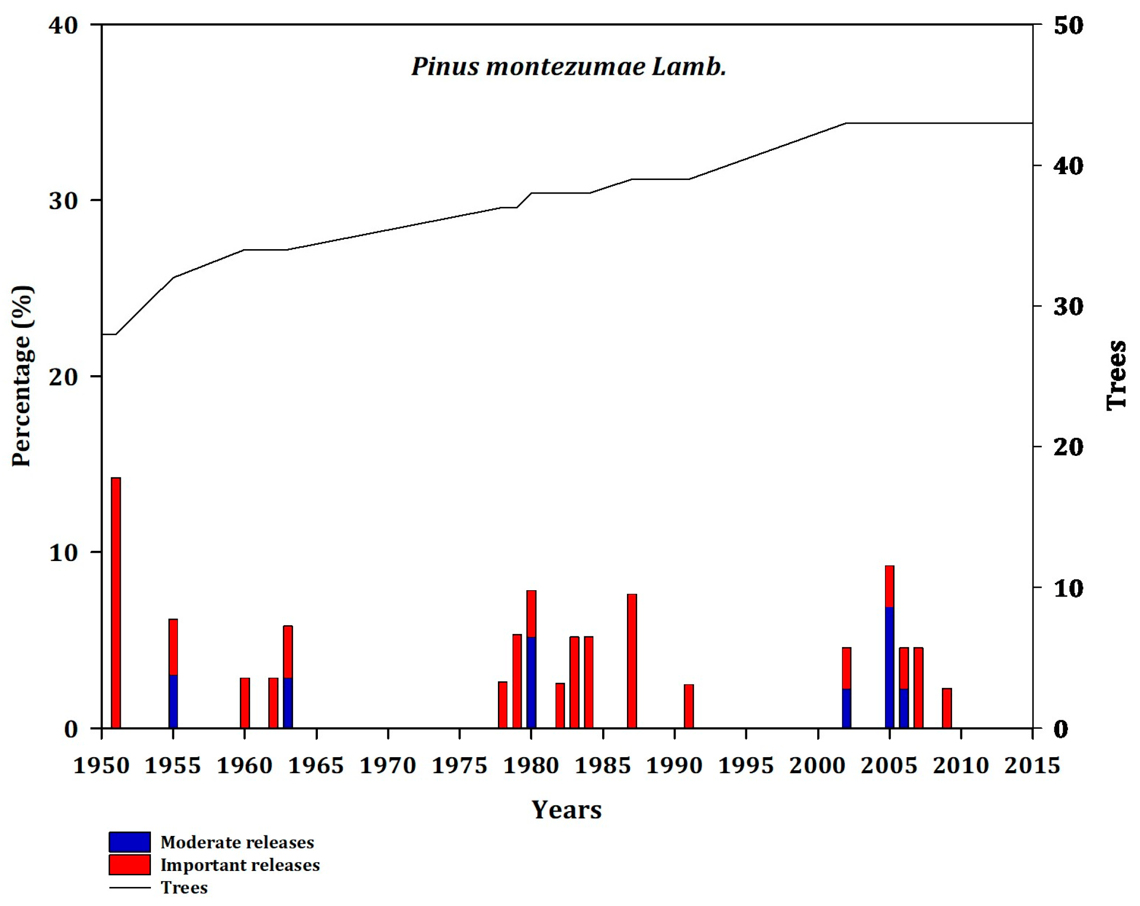
CUE and JAC at the same site (Güemes, Tamaulipas) showed the same pattern of release, unlike Pov and Ptn. MES showed more frequent major releases (>50%) (Appendix B, Figure A5, Figure A6 and Figure A7). MOR experienced disturbances continuously during 1976–2003, with the highest proportion of trees showing strong releases in 1980 and 1993, while at POZ there were moderate releases (Appendix B, Figure A8).
In the sites of central Mexico, a greater number of trees responded moderately to disturbance. Pts, Phm, and Plu evidenced disturbance only in 1957, 1960, 1961, and 1962 (Appendix B, Figure A9, Figure A10 and Figure A11).
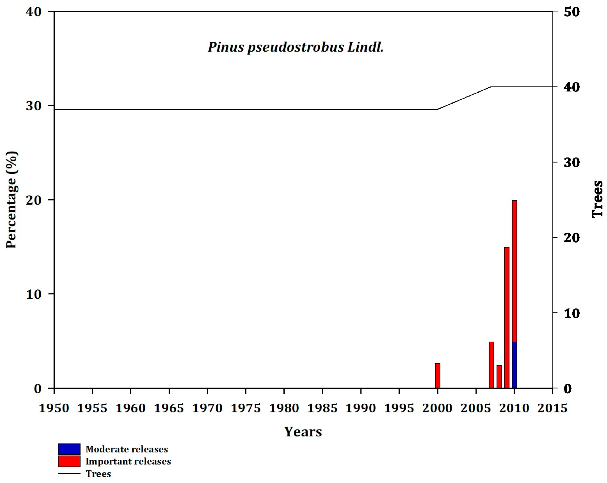
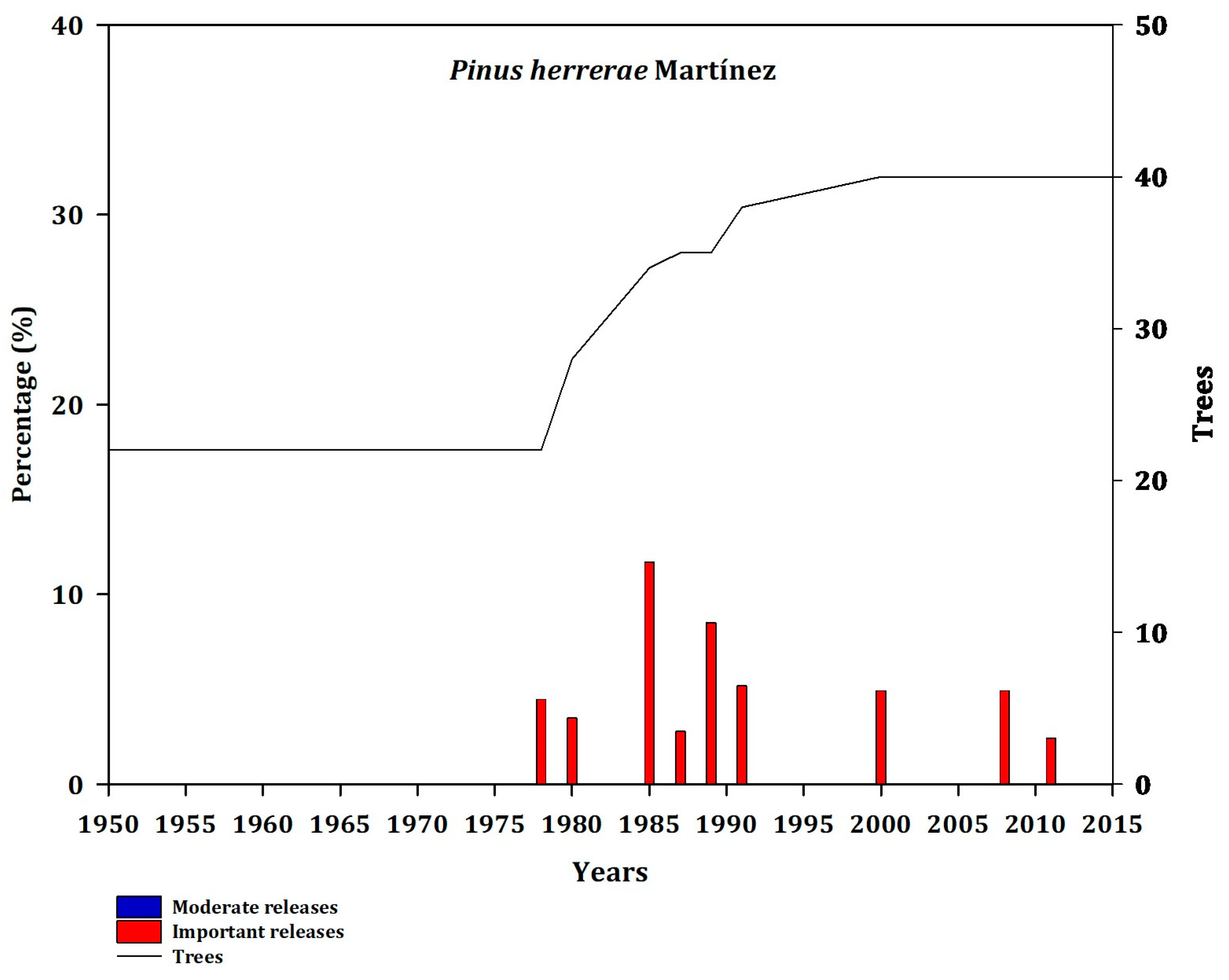
At sites neighboring the Pacific Ocean, Pce showed medium intensity disturbance (Appendix B, Figure A12). Jdp showed a strong release in 1976, but a lower incidence in number of trees (Appendix B, Figure A13). Pdu recorded a low rate of forest disturbance from 1973 to 2007 (Appendix B, Figure A14). Phe presented moderate disturbances from 1978 to 2011 (Appendix B, Figure A15). Poj had a lower intensity from 2005 to 2011 (Appendix B, Figure A16).
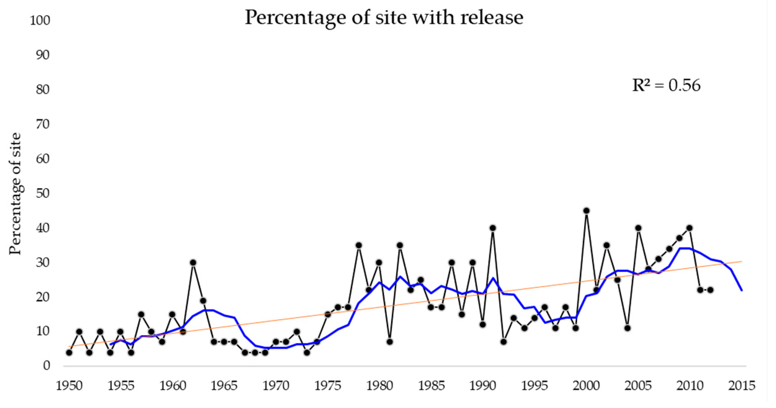
Our results indicate that disturbance frequency increased during the second study period (1981–2010) (Figure 3). Nevertheless, some sites had similar disturbance frequencies over both periods (e.g., LAG, RAN, or COR; see Appendix B). In particular, sites in northeastern Mexico presented a greater intensity in releases. In contrast, the sites of central Mexico showed a moderate change in disturbances between the two periods studied.
The SPEI dynamic indicates differences in drought frequency and intensity between the Pacific Ocean and the Gulf of Mexico, especially during the last two decades (Figure 4). Thus, the trees growing near the Gulf of Mexico differed in release events, which may reflect their differential responsiveness to precipitation episodes (e.g., hurricanes), particularly from 1996 onwards.
4. Discussion
To our knowledge, this study is the first of its kind in Mexico to identify disturbances. We identified past disturbances in 13 species of young Mexican conifers along a diverse spatial ecological gradient. We analyzed the release of ring width growth in each species over a range of years from 1950 to 2010. We did not examine the effects of stand characteristics (Table 1) on apparent disturbances, a theme that merits further research.
4.1. Identification of Temporal Disturbance
Variability was found in the reconstruction of disturbances among the 13 species studied. The ring-width data showed widespread disturbances for the period 1950 to 2010, suggesting complex disturbance patterns within and among the studied species, and supporting the previous reports of other authors [31]. Species exhibited different temporal patterns of disturbance represented by the growth failures observed.
Given that these forests are unevenly aged, this indicates that they have not been disturbed by a single catastrophic event that completely killed the stand. The frequency and intensity of the releases detected here indicates that there have only been episodes of gap forming disturbances. However, the short temporal scale of the study of these species is inconclusive in terms of disturbances, since the previous occurrence of these events (prior to 1950) remains unknown. According to our results (Figure 4), we hypothesize that disturbances in Mexico will be associated with the combination of drought and other climatological phenomena, such as hurricanes or landslides caused by heavy rains, as well as pathogens and diseases associated with drought and fire regimes. Further research on these phenomena and their relationships to the disturbances is therefore vital at the site level as it is impossible to capture such complexity over a large area without long-term observation and detailed records.
4.2. Spatial Characterization of Disturbances
Species found in the eastern sites presented a higher frequency of disturbance compared to those in the west and center. This was most evident during the period from 1950 to 1980, and was consistent with a global study indicating that the increased frequency and severity of droughts due to climate change has become the main factor affecting tree growth. Another similar result was the change in response as a function of the period of analysis, since differences in growth response to climatic conditions and drought were found in the periods 1950–1980 and 1981–2010. This suggests that climate variability is an important factor to consider when reconstructing disturbance regimes. Our results suggest specific interactions between disturbance trends and seasonal hydroclimate variability.
Temporally, disturbances were recurrent, but only severe in certain years. This reconstruction suggested that these disturbances were infrequent but more severe, a finding that was consistent with that reported in studies from other countries [10]. This is attributed to the response of these species to large-scale natural disturbances such as hurricanes [18] and circulatory phenomena such as ENSO (El Niño Southern Oscillation) [32,33]. There is consistent evidence of spatially extended perturbations that synchronously affect different biome types. Several of the reconstructions of regional-scale disturbances are associated with intense regional drought events triggered by the variability of ENSO in the Pacific Ocean [31]. Across the species, we found that some explain the disturbance through geographic proximity, while others respond differently to disturbances. This has ecological implications for forest successional processes and structural characteristics [34]. In other words, forest composition is determined by resistance or resilience to disturbance, which provides a tool for managers to shape their silvicultural regimes [12].
The spatial perspective shows certain geographic patterns are attributed to the occurrence of site-level disturbances. However, different species at the same site showed differences in the occurrence of disturbances. This could be explained by the fact that frequent and less severe natural forest disturbances generally occur at smaller spatial scales [35]. From a temporal perspective, Figure 2 shows an increase in disturbance. This indicates a warning signal in the vegetation dynamics that deserves further research in order to elucidate the ecological or anthropogenic mechanisms underlying these disturbances. In general, species from sites closer to the Gulf of Mexico (between 95° and 100° W) were disturbed more frequently than those closer to the Pacific Ocean (between 100° and 105° W). Although we did not investigate the causes of disturbance in depth, our dendroecological approach showed a clear differentiation in responses to disturbances between the Gulf of Mexico and Pacific Ocean regions.
We found that in Gulf of Mexico there are, in general, fewer droughts and drought and wet periods alternate. However, there have been two relatively long and intense drought periods (one in 1960 and one before 2000), which did not occur in the Pacific. This intense drought could induce tree mortality. Thus, we suggest that the higher intensity of detected releases in the Gulf of Mexico may be related to drought [36]. In addition, the Gulf of Mexico is significantly more affected by hurricane activity, and thus we suggest that the combination of drought and hurricanes is mainly responsible for forest disturbances in this area (see Appendix C to analyze relationships between geographic space and environmental influences on the disturbances).
We can speculate that the climate–growth relationships are acting to regulate the disturbances in each zone. Thus, the west is controlled by the North American summer monsoon related to El Niño [37]. The positive correlations between growth and SPEI confirm that El Niño events are associated with radial growth. On the other hand, the forests of the east appear to present promising opportunities under the occurrence of hurricanes. Moreover, both regions offer different microsite conditions, including topography, genetic load, seasonal growth, etc., that merit further investigation. Previous studies have documented that the presence of disturbances (hurricanes) has an impact on Earlywood (EW) and Latewood (LW) anatomical characteristics [38]. We therefore recommend further investigation with higher temporal resolution proxies (EW, LW) for future studies. It is known that the seasonal responses of trees can convey a fingerprint of disturbance that is not reflected in the total ring width [39].
Another limitation of our study could be the short duration of the analysis period, and data available in the International Tree-Ring Data Bank (ITRDB) could be utilized to complement the temporal perspective [6]. Expanding the temporal perspective could greatly benefit the scope of our study, as could explaining the causes of such disturbances. Understanding their dynamics and examining their causes in the future will allow predictions to be made with respect to migration, decline, and mortality episodes, including tree mortality.
Other factors for consideration should include species resilience, recovery, and plasticity since, as seen here, there are differences in the frequency and severity of disturbances found among coexisting species. Forest resilience has been used to measure the severity of disturbances such as drought and is a good indicator of forest composition [40]. Studies of intraspecific genetic variation and phenotypic plasticity are also essential in order to estimate the vulnerability of forest species to drought [41,42]. Further research is recommended in order to test these arguments.
The histogram of detected growth releases provided insights into the disturbance regime. Thus, the disturbances have consequences for forest development due to the fact that they interrupt continuous succession and alter growth rates. This has direct implications in terms of redefining the concept of natural succession, which in turn impacts the composition and structure of species. This tool should be integrated into the portfolio of the forest manager, as a complement to inventory data. For example, the estimation of disturbance frequency produced in this study is crucial for decision-making because the studied species are subjected to forest management and logging [21,39]; it has been documented that the age of rotation within forest management should not exceed the frequency of the disturbances [7].
5. Conclusions
Here, we investigated the recording of spatial and temporal disturbances by contemporary conifer species representative of forest ecosystems in Mexico.
The results suggest that forest disturbances follow a spatial and temporal trend. It is difficult to reach a definitive conclusion and to generalize regarding the multifactorial causes of forest disturbances across a large study area. Although the influence of anthropogenic disturbances has already been demonstrated, in this study it is evident that climate and large-scale circulatory patterns influence the release rates. Overall, disturbances appear to follow an increasing rate from 2000 onwards. The proxies used in this study produced parameters that improve our understanding of forest dynamics and should be considered in vegetation dynamics models to reduce uncertainty in the face of climate vulnerability. Our approach constitutes a suitable route for identifying disturbances as parameters of great importance that can act to configure the structure, composition, and function of forest ecosystems.
Author Contributions
M.P.-G. conceived and designed the experiment, led the data analysis, and wrote and edited the original manuscript. D.S.P.-M. processed data, conducted formal analyses and utilized software. J.A. conducted formal analyses and wrote the manuscript. J.A.M.R. conducted formal analyses, visualization and edited the final version of the manuscript. All authors have read and agreed to the published version of the manuscript.
Funding
We thank CONACYT for the funding provided through project A1-S-21471, COCYTED, and DendroRed, (http://dendrored.ujed.mx; accessed on 11 November 2022). J.A. was supported by Research Grants LTAUSA19137 (program INTER-EXCELLENCE, subprogram INTER-ACTION) provided by the Czech Ministry of Education, Youth and Sports, 23-05272S of the Czech Science Foundation, and long-term research development project RVO 67985939 of the Institute of Botany of the Czech Academy of Sciences.
Acknowledgments
We thank Andrés Cruz Cruz (El Capy), Ciriaco Rangel Alonso, David Ezequiel Chávez Martínez, Emmanuel Cruz Canela, Esteban Casillas Núñez, Feliciano González Ávila, Gustavo Castañeda Rosales, Esaúl López Mendoza, Leonel Carmona Duarte, Mauro Ramírez Alavez, Sergio Ruíz Soto, José Alberto Ramos Caballero, José Antonio Álvaro Méndez, José Cruz Delgado Campos, Julio Godínez Rojo, Adrián Jesús Mendoza Herrera, Maximiliano García Flores, Miguel Hernández Espejel, Oscar Alfredo Díaz Carrillo, Roberto Carlos Valadez Castro, José Jesús García Cruz, José Remedios Hernández Hernández, Ramiro Martínez Acosta, Eduardo Pánuco Rivera, Rigoberto González Cubas, Humberto López Alejandro, Mariana García Flores, Alfredo Hernández Camacho, Sergio Hernández Sánchez, Joel Antonio Loya García, Eduardo Daniel Vivar Vivar, and Rubén Darío Appel Espinoza for the support provided for data collection. We thank Marcos González-Cásares and Eduardo Vivar-Vivar, for their support on previous versions of the manuscript.
Conflicts of Interest
The authors declare no conflict of interest.
Abbreviations
Ring width index (RWI); ring width length (RWL); tree ring width (TRW); correlation between trees (Rbt); subsample signal strength (SSS); expressed population signal (EPS); kernel density estimation (KDE); annual heat-moisture index (AHMI); Pov Pinus oocarpa Schiede ex Schltdl. Pay Pinus ayacahuite Ehren. var. ayacahuite. Phc Pinus hartwegii Lindl (Coahuila). Pmo Pinus montezumae Lamb. Ppa Pinus patula Schltdl. et Cham. Pse Pinus pseudostrobus Lindl. Ptn Pinus teocote Schiede ex Schltdl (Nuevo León). Pts Pinus teocote Schiede ex Schltdl (San Luis). Phm Pinus hartwegii Lindl (México). Plu Pinus lumholtzii B.L. Rob & Fernald. Jdp Juniperus deppeana Steud. Poj Pinus oocarpa Schiede ex Schltdl. Pdu Pinus durangensis Martínez. Phe Pinus herrerae Martínez. Pce Pinus cembroides subsp. Lagunae (Rob. Pass.) D.K. Bailey.
Appendix A
In this section, we provide additional information of dendrochronological statistics and residual chronologies of the studied species.

Table A1.
Dendrochronological statistics of the sampled species.
| Site Name | Spp | n (nc) | TRW ± sd | Years ± sd | Rbt | EPS | Period |
|---|---|---|---|---|---|---|---|
| Pacific Ocean (PO) | |||||||
| La Laguna = LAG | Pce | 15 (30) | 1.28 ± 0.07 | 66 ± 5 | 0.32 | 0.87 | 1970–2019 |
| Potrero de Mulas = MUL | Poj | 20 (40) | 1.57 ± 0.05 | 43 ± 1 | 0.41 | 0.96 | 1987–2021 |
| Alto de la Lagunita = ALT | Phe | 20 (40) | 2.36 ± 0.12 | 51 ± 4 | 0.43 | 0.97 | 1982–2021 |
| Papanton = PAP | Jdp | 16 (33) | 2.16 ± 0.19 | 35 ± 2 | 0.54 | 0.96 | 1986–2020 |
| Cerro del Bravo = BRA | Plu | 18 (36) | 1.38 ± 0.09 | 74 ± 5 | 0.45 | 0.94 | 1917–2020 |
| Alto de la Lagunita = ALT | Pdu | 20 (40) | 1.68 ± 0.08 | 52 ± 2 | 0.3 | 0.94 | 1992–2021 |
| Gulf of Mexico (GM) | |||||||
| La Mesa = MES | Ptn | 20 (40) | 4.16 ± 0.13 | 40 ± 1 | 0.52 | 0.97 | 1977–2020 |
| Cerro El Morro = MOR | Phc | 15 (31) | 1.61 ± 0.18 | 73 ± 7 | 0.48 | 0.97 | 1987–2021 |
| Orillas de Ocotal Chico = OCO | Pov | 16 (33) | 3.16 ± 0.20 | 28 ± 0.5 | 0.26 | 0.9 | 1986–2020 |
| El Jacalón = JAC | Ppa | 20 (41) | 2.46 ± 0.09 | 67 ± 2 | 0.49 | 0.97 | 1952–2020 |
| La Cueva = CUE | Pmo | 20 (43) | 2.01 ± 0.11 | 72 ± 3 | 0.38 | 0.95 | 1937–2020 |
| Rancho Joyas del Durazno = RAN | Pts | 19 (38) | 2.50 ± 0.15 | 44 ± 2 | 0.59 | 0.97 | 1970–2020 |
| La Mesa = MES | Pse | 20 (40) | 4.34 ± 0.19 | 32 ± 1 | 0.42 | 0.95 | 1983–2020 |
| Mexico Center (MC) | |||||||
| Corral de los Borregos= COR | Pay | 20 (40) | 2.92 ± 0.11 | 56 ± 3 | 0.33 | 0.93 | 1959–2020 |
| Pozuelos = POZ | Phm | 13 (27) | 1.64 ± 0.11 | 65 ± 5 | 0.26 | 0.86 | 1975–2019 |
where Spp = species, n = no. of trees, nc = no. of cores, TRW = tree-ring width, Years = no. of years, Rbt = correlation between trees, and EPS = expressed population signal.
Figure A1.
Ring width residual chronologies (left y-axis) and subsample signal strength (right y-axis) of species (a) (Jde) Juniperus deppeana Steud., (b) (Pay) Pinus ayacahuite Ehren. Variedad ayacahuite., (c) (Pce) Pinus cembroides subsp. Lagunae (Rob. Pass.) D.K. Bailey., (d) (Pdu) Pinus durangensis Martínez., (e) (Phc) Pinus hartwegii Lindl. (Coahuila), (f) (Phe) Pinus herrerae Martínez., (g) (Phm) Pinus hartwegii Lindl. (Estado de México), (h) (Plu) Pinus lumholtzii B.L. Rob & Fernald., (i) (Pmo) Pinus montezumae Lamb., (j) (Poj) Pinus oocarpa Schiede ex Schltdl. (Jalisco), (k) (Pov) Pinus oocarpa Schiede ex Schltdl. (Veracruz), (l) (Ppa) Pinus patula Schltdl. et Cham., (m) (Pse) Pinus pseudostrobus Lindl., (n) (Ptn) Pinus teocote Schiede ex Schltdl. (Nuevo León), (o) (Pts) Pinus teocote Schiede ex Schltdl. (San Luis Potosí). LAG = La Laguna, MUL = Potrero de Mulas, ALT = Alto de la Lagunita, PAP = Papanton, BRA = Cerro del Brabo, MES, La Mesa, MOR = Cerro El Moro, OCO = Orillas de Ocotal Chico, JAC = Jacalón, CUE = La Cueva, RAN = Rancho Joyas del Durazno, COR = Corral de los Borregos, POZ = Pozuelos, PO = the Pacific Ocean, GM = the Gulf of Mexico, and MC = the Mexico Center.


Appendix B
Figure A2.
Frequency of disturbance in Pmo (CUE; GM). Moderate releases 20% to 49.99% (blue bars) and major (important) releases >50% (red bars). The line represents the number of trees that showed a decrease in growth as a function of releases.
Figure A2.
Frequency of disturbance in Pmo (CUE; GM). Moderate releases 20% to 49.99% (blue bars) and major (important) releases >50% (red bars). The line represents the number of trees that showed a decrease in growth as a function of releases.

Figure A3.
Frequency of disturbance in Ppa (JAC; GM). Moderate releases 20% to 49.99% (blue bars) and major (important) releases >50% (red bars). The line represents the number of trees that showed a decrease in growth as a function of releases.
Figure A3.
Frequency of disturbance in Ppa (JAC; GM). Moderate releases 20% to 49.99% (blue bars) and major (important) releases >50% (red bars). The line represents the number of trees that showed a decrease in growth as a function of releases.

Figure A4.
Frequency of disturbance in Phc (MOR; GM). Moderate releases 20% to 49.99% (blue bars) and major (important) releases >50% (red bars). The line represents the number of trees that showed a decrease in growth as a function of releases.
Figure A4.
Frequency of disturbance in Phc (MOR; GM). Moderate releases 20% to 49.99% (blue bars) and major (important) releases >50% (red bars). The line represents the number of trees that showed a decrease in growth as a function of releases.

Figure A5.
Frequency of disturbance in Pov (OCO; GM). Moderate releases 20% to 49.99% (blue bars) and major (important) releases >50% (red bars). The line represents the number of trees that showed a decrease in growth as a function of releases.
Figure A5.
Frequency of disturbance in Pov (OCO; GM). Moderate releases 20% to 49.99% (blue bars) and major (important) releases >50% (red bars). The line represents the number of trees that showed a decrease in growth as a function of releases.

Figure A6.
Frequency of disturbance in Ptn (MES; GM). Moderate releases 20% to 49.99% (blue bars) and major (important) releases >50% (red bars). The line represents the number of trees that showed a decrease in growth as a function of releases.
Figure A6.
Frequency of disturbance in Ptn (MES; GM). Moderate releases 20% to 49.99% (blue bars) and major (important) releases >50% (red bars). The line represents the number of trees that showed a decrease in growth as a function of releases.

Figure A7.
Frequency of disturbance in Pse (MES; GM). Moderate releases 20% to 49.99% (blue bars) and major (important) releases >50% (red bars). The line represents the number of trees that showed a decrease in growth as a function of releases.
Figure A7.
Frequency of disturbance in Pse (MES; GM). Moderate releases 20% to 49.99% (blue bars) and major (important) releases >50% (red bars). The line represents the number of trees that showed a decrease in growth as a function of releases.

Figure A8.
Frequency of disturbance in Pay (COR; MC). Moderate releases 20% to 49.99% (blue bars) and major (important) releases >50% (red bars). The line represents the number of trees that showed a decrease in growth as a function of releases.
Figure A8.
Frequency of disturbance in Pay (COR; MC). Moderate releases 20% to 49.99% (blue bars) and major (important) releases >50% (red bars). The line represents the number of trees that showed a decrease in growth as a function of releases.

Figure A9.
Frequency of disturbance in Pts (RAN; GM). Moderate releases 20% to 49.99% (blue bars) and major (important) releases >50% (red bars). The line represents the number of trees that showed a decrease in growth as a function of releases.
Figure A9.
Frequency of disturbance in Pts (RAN; GM). Moderate releases 20% to 49.99% (blue bars) and major (important) releases >50% (red bars). The line represents the number of trees that showed a decrease in growth as a function of releases.

Figure A10.
Frequency of disturbance in Phm (POZ; MC). Moderate releases 20% to 49.99% (blue bars) and major (important) releases >50% (red bars). The line represents the number of trees that showed a decrease in growth as a function of releases.
Figure A10.
Frequency of disturbance in Phm (POZ; MC). Moderate releases 20% to 49.99% (blue bars) and major (important) releases >50% (red bars). The line represents the number of trees that showed a decrease in growth as a function of releases.

Figure A11.
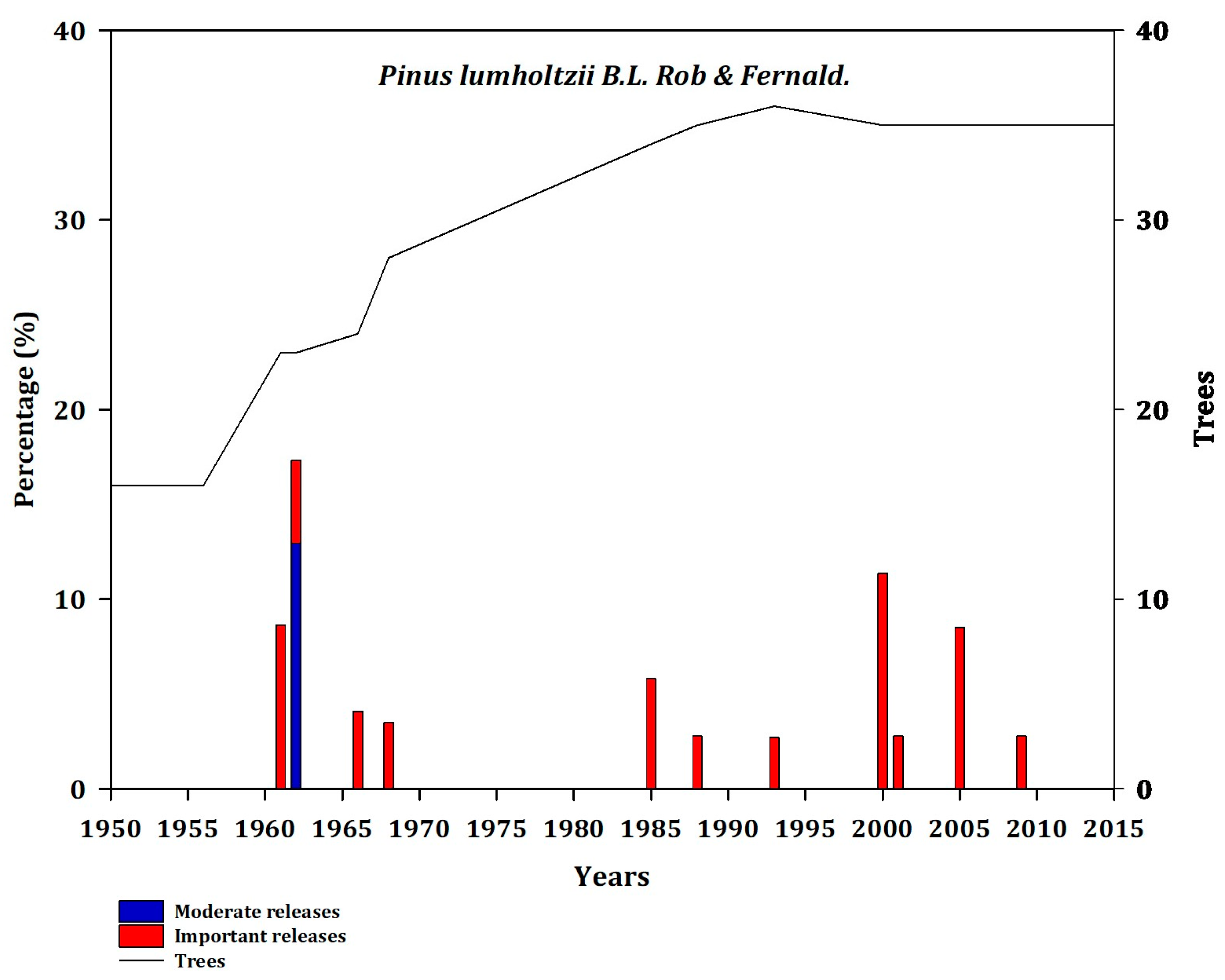
Frequency of disturbance in Plu (BRA; PO). Moderate releases 20% to 49.99% (blue bars) and major (important) releases >50% (red bars). The line represents the number of trees that showed a decrease in growth as a function of releases.
Figure A11.
Frequency of disturbance in Plu (BRA; PO). Moderate releases 20% to 49.99% (blue bars) and major (important) releases >50% (red bars). The line represents the number of trees that showed a decrease in growth as a function of releases.

Figure A12.
Frequency of disturbance in Pce (LAG; PO). Moderate releases 20% to 49.99% (blue bars) and major (important) releases >50% (red bars). The line represents the number of trees that showed a decrease in growth as a function of releases.
Figure A12.
Frequency of disturbance in Pce (LAG; PO). Moderate releases 20% to 49.99% (blue bars) and major (important) releases >50% (red bars). The line represents the number of trees that showed a decrease in growth as a function of releases.

Figure A13.
Frequency of disturbance in Jdp (PAP; PO). Moderate releases 20% to 49.99% (blue bars) and major (important) releases >50% (red bars). The line represents the number of trees that showed a decrease in growth as a function of releases.
Figure A13.
Frequency of disturbance in Jdp (PAP; PO). Moderate releases 20% to 49.99% (blue bars) and major (important) releases >50% (red bars). The line represents the number of trees that showed a decrease in growth as a function of releases.

Figure A14.
Frequency of disturbance in Pdu (ALT; PO). Moderate releases 20% to 49.99% (blue bars) and major (important) releases >50% (red bars). The line represents the number of trees that showed a decrease in growth as a function of releases.
Figure A14.
Frequency of disturbance in Pdu (ALT; PO). Moderate releases 20% to 49.99% (blue bars) and major (important) releases >50% (red bars). The line represents the number of trees that showed a decrease in growth as a function of releases.

Figure A15.
Frequency of disturbance in Phe (ALT; PO). Moderate releases 20% to 49.99% (blue bars) and major (important) releases >50% (red bars). The line represents the number of trees that showed a decrease in growth as a function of releases.
Figure A15.
Frequency of disturbance in Phe (ALT; PO). Moderate releases 20% to 49.99% (blue bars) and major (important) releases >50% (red bars). The line represents the number of trees that showed a decrease in growth as a function of releases.

Figure A16.
Frequency of disturbance in Poj (MUL; PO). Moderate releases 20% to 49.99% (blue bars) and major (important) releases >50% (red bars). The line represents the number of trees that showed a decrease in growth as a function of releases.
Figure A16.
Frequency of disturbance in Poj (MUL; PO). Moderate releases 20% to 49.99% (blue bars) and major (important) releases >50% (red bars). The line represents the number of trees that showed a decrease in growth as a function of releases.

Appendix C
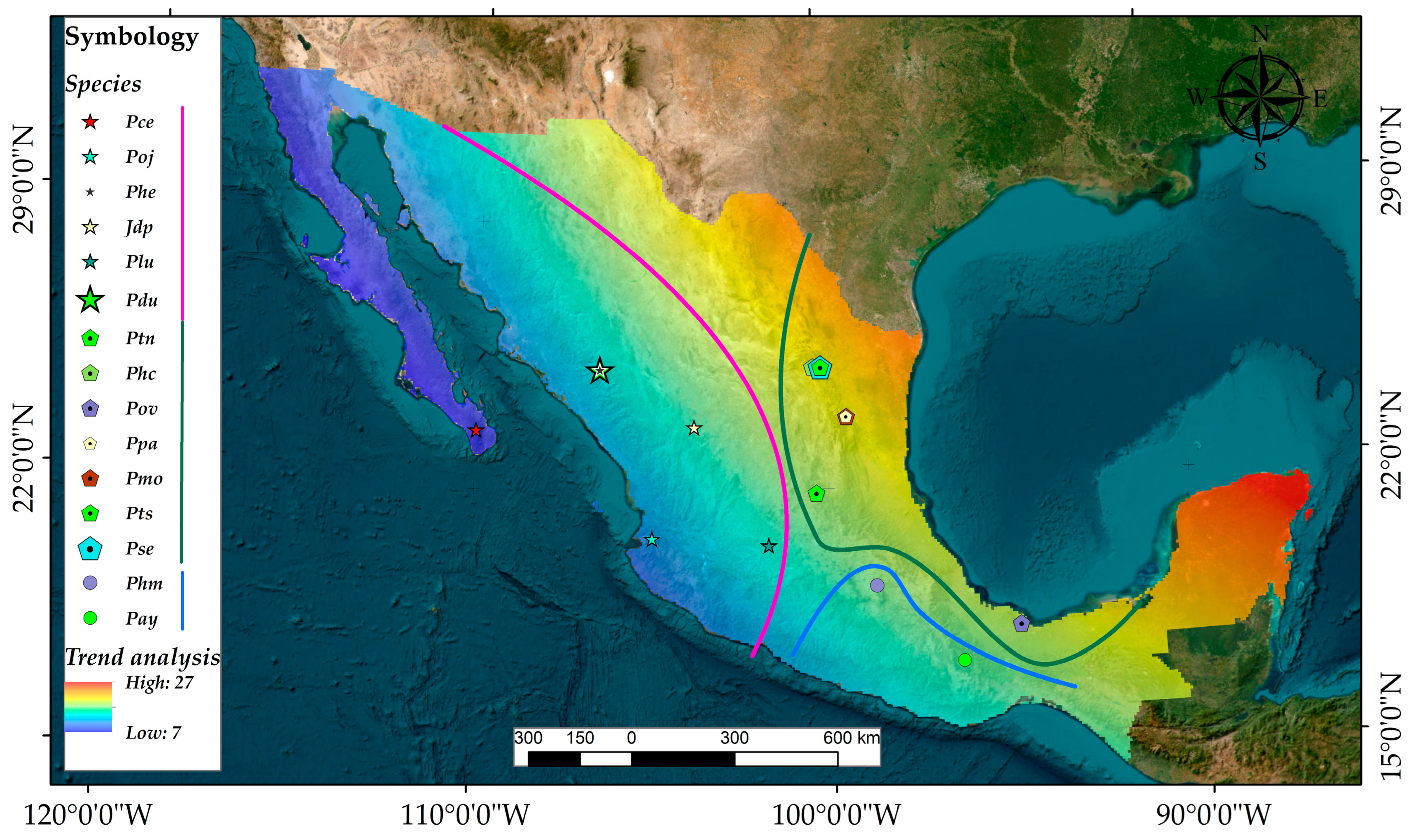
Figure A17.
Map showing the location of each sampled tree species. A trend surface analysis was conducted to test for the spatial effect on releases. We used a first-order polynomial to capture coarse-scale patterns in the data of percentage releases, based on elevation and distance. The color range denotes the quantification of the role of space on disturbance varying from low (blue) to high (red), indicating that proximity to the Gulf of Mexico is more strongly associated with releases than proximity to the Pacific Ocean.

References
- Nguyen, T.; Jones, S.; Soto-Berelov, M.; Haywood, A.; Hislop, S. A spatial and temporal analysis of forest dynamics using Landsat time-series. Remote Sens. Environ. 2018, 217, 461–475. [Google Scholar] [CrossRef]
- McDowell, N.; Allen, C.; Anderson-Teixeira, K.; Aukema, B.; Bond-Lamberty, B.; Chini, L.; Clark, J.; Dietze, M.; Grossiord, C.; Hanbury-Brown, A.; et al. Pervasive shifts in forest dynamics in a changing world. Science 2020, 368, 9463. [Google Scholar] [CrossRef]
- Canelles, Q.; Aquilué, N.; James, P.; Lawler, J.; Brotons, L. Global review on interactions between insect pests and other forest disturbances. Landsc. Ecol. 2021, 36, 945–972. [Google Scholar] [CrossRef]
- Seidl, R.; Thom, D.; Kautz, M.; Martin-Benito, D.; Peltoniemi, M.; Vacchiano, G.; Wild, J.; Ascoli, D.; Petr, M.; Honkaniemi, J.; et al. Forest disturbances under climate change. Nat. Clim. Chang. 2017, 7, 395–402. [Google Scholar] [CrossRef]
- Kleinman, J.; Goode, J.; Fries, A.; Hart, J. Ecological consequences of compound disturbances in forest ecosystems: A systematic review. Ecosphere 2019, 10, e02962. [Google Scholar] [CrossRef]
- Altman, J. Tree-ring-based disturbance reconstruction in interdisciplinary research: Current state and future directions. Dendrochronologia 2020, 63, 125733. [Google Scholar] [CrossRef]
- Lorimer, C.; Frelich, L. A methodology for estimating canopy disturbance frequency and intensity in dense temperate forests. Can. J. For. Res. 1989, 19, 651–663. [Google Scholar] [CrossRef]
- Nowacki, G.; Abrams, M. Radial growth averaging criteria for reconstructing disturbance histories from presettlement origin oaks. Ecol. Monogr. 1997, 67, 225–249. [Google Scholar] [CrossRef]
- Trotsiuk, V.; Pederson, N.; Druckenbrod, D.; Orwig, D.; Bishop, D.; Barker-Plotkin, A.; Fraver, S.; Martin-Benito, D. Testing the efficacy of tree-ring methods for detecting past disturbances. For. Ecol. Manag. 2018, 425, 59–67. [Google Scholar] [CrossRef]
- Altman, J.; Fibich, P.; Leps, J.; Uemura, S.; Harad, T.; Dolezal, J. Linking spatiotemporal disturbance history with tree regeneration. Perspect. Plant Ecol. Evol. Syst. 2016, 21, 1–13. [Google Scholar] [CrossRef]
- Sánchez-Pinillos, M.; Leduc, A.; Ameztegui, A.; Kneeshaw, D.; Lloret, F.; Coll, L. Resistance, resilience or change: Post-disturbance dynamics of boreal forests after insect outbreaks. Ecosystems 2019, 22, 1886–1901. [Google Scholar] [CrossRef]
- Čada, V.; Trotsiuk, V.; Janda, P.; Mikoláš, M.; Bače, R.; Nagel, T.; Morrissey, R.; Tepley, A.; Vostarek, O.; Begović, K.; et al. Quantifying natural disturbances using a large-scale dendrochronological reconstruction to guide forest management. Ecol. Appl. 2020, 30, e02189. [Google Scholar] [CrossRef]
- Maes, S.L.; Vannoppen, A.; Altman, J.; van den Bulcke, J.; Decocq, G.; de Mil, T.; Depauw, L.; Landuyt, D.; Perring, M.P.; van Acker, J.; et al. Evaluating the robustness of three ring-width measurement methods for growth release reconstruction. Dendrochronologia 2017, 46, 67–76. [Google Scholar] [CrossRef]
- Druckenbrod, D.; Pederson, N.; Rentch, J.; Cook, E. A comparison of times series approaches for dendroecological reconstructions of past canopy disturbance events. For. Ecol. Manag. 2013, 302, 23–33. [Google Scholar] [CrossRef]
- Kuosmanen, N.; Čada, V.; Halsall, K.; Chiverrell, R.; Schafstall, N.; Kuneš, P.; Boyle, J.; Knížek, M.; Appleby, P.; Svoboda, M.; et al. Integration of dendrochronological and palaeoecological disturbance reconstructions in temperate mountain forests. For. Ecol. Manag. 2020, 475, 118413. [Google Scholar] [CrossRef]
- Altman, J.; Doležal, J.; Černý, T.; Song, J. Forest response to increasing typhoon activity on the Korean peninsula: Evidence from oak tree-rings. Glob. Chang. Biol. 2013, 19, 498–504. [Google Scholar] [CrossRef] [PubMed]
- Acosta-Hernández, A.; Pompa-García, M.; Camarero, J.J. An updated review of dendrochronological investigations in Mexico, a megadiverse country with a high potential for tree-ring sciences. Forests 2017, 8, 160. [Google Scholar] [CrossRef]
- Maass, M.; Ahedo-Hernández, R.; Araiza, S.; Verduzco, A.; Martínez-Yrízar, A.; Jaramillo, V.; Parker, G.; Pascual, F.; García-Méndez, G.; Sarukhán, J. Long-term (33 years) rainfall and runoff dynamics in a tropical dry forest ecosystem in western Mexico: Management implications under extreme hydrometeorological events. For. Ecol. Manag. 2018, 426, 7–17. [Google Scholar] [CrossRef]
- Cerano-Paredes, J.; Villanueva-Díaz, J.; Vázquez-Selem, L.; Cervantes-Martínez, R.; Esquivel-Arriaga, G.; Guerra-de la Cruz, V.; Fulé, P.Z. Régimen histórico de incendios y su relación con el clima en un bosque de Pinus hartwegii al norte del estado de Puebla, México. Bosque Valdivia 2016, 37, 389–399. [Google Scholar] [CrossRef]
- González-Cásares, M.; Pompa-García, M.; Padilla-Martínez, J. Pith eccentricity, basal area increments and disturbances inferred from tree-ring growth. Tree-Ring Res. 2022, 78, 25–35. [Google Scholar] [CrossRef]
- Vivar-Vivar, E.; Pompa-García, M.; Rodríguez-Trejo, D.; Leyva-Ovalle, A.; Wehenkel, C.; Carrillo-Parra, A.; García-Montiel, E.; Moreno-Anguiano, O. Drought responsiveness in two Mexican conifer species forming young stands at high elevations. For. Syst. 2021, 30, e012. [Google Scholar] [CrossRef]
- Poorter, L.; Bongers, F.; Aide, M.; Almeyda, A.; Balvanera, P.; Becknell, J.; Boukili, V.; Brancalion, P.; Broadbent, E.; Chazdon, R.; et al. Biomass resilience of Neotropical secondary forests. Nature 2016, 530, 211–214. [Google Scholar] [CrossRef]
- Gernandt, D.; Pérez-de la Rosa, J. Biodiversity of Pinophyta (conifers) in Mexico. Rev. Mex. Biodivers. Supl. 2014, 85, S126–S133. [Google Scholar] [CrossRef]
- Pompa-García, M.; Sigala, J.; Jurado, E. Some tree species of ecological importance in Mexico: A documentary review. Rev. Chapingo Ser. Cienc. For. Ambiente 2017, 23, 185–219. [Google Scholar] [CrossRef]
- Cook, E.; Holmes, R. Users manual for program ARSTAN. In Tree-Ring Chronologies of Western North America: California, Eastern Oregon and Northern Great Basin; Holmes, R.L., Adams, R.K., Fritts, H.C., Eds.; Laboratory of Tree-Ring Research: Tucson, AZ, USA, 1986; pp. 50–65. Available online: http://hdl.handle.net/10150/304672 (accessed on 10 April 2022).
- Wigley, T.; Briffa, K.; Jones, P. On the average value of correlated time series, with applications in dendroclimatology and hydrometeorology. J. Appl. Meteorol. 1984, 23, 201–213. [Google Scholar] [CrossRef]
- Black, B.; Abrams, M. Use of boundary line growth patterns as a basis for dendroecological release criteria. Ecol. Appl. 2003, 13, 1733–1749. [Google Scholar] [CrossRef]
- Altman, J.; Fibich, P.; Dolezal, J.; Aakala, T. TRADER: A package for tree ring analysis of disturbance events in R. Dendrochronologia 2014, 32, 107–112. [Google Scholar] [CrossRef]
- R Core Team. R: A Language and Environment for Statistical Computing; R Foundation for Statistical Computing: Vienna, Austria, 2021; Available online: https://www.R-project.org (accessed on 13 April 2022).
- Monjarás-Vega, N.; Briones-Herrera, C.I.; Vega-Nieva, D.; Calleros-Flores, E.; Corral-Rivas, J.; López-Serrano, P.M.; Pompa-García, M.; Rodriguez-Trejo, D.A.; Carrillo-Parra, A.; González-Cabán, A.; et al. Predicting forest fire kernel density at multiple scales with geographically weighted regression in Mexico. Sci. Total Environ. 2020, 718, 137313. [Google Scholar] [CrossRef] [PubMed]
- Baker, P.; Bunyavejchewin, S. Complex historical disturbance regimes shape forest dynamics across a seasonal tropical landscape in western Thailand. In Dendroecology; Springer: Cham, Switzerland, 2017; pp. 75–96. [Google Scholar] [CrossRef]
- Pompa-García, M.; Miranda-Aragón, L.; Aguirre-Salado, C. Tree growth response to ENSO in Durango, Mexico. Int. J. Biometeorol. 2014, 59, 89–97. [Google Scholar] [CrossRef]
- González-Cásares, M.; Pompa-García, M.; Camarero, J. Differences in climate–growth relationship indicate diverse drought tolerances among five pine species coexisting in Northwestern Mexico. Trees 2017, 31, 531–544. [Google Scholar] [CrossRef]
- Carter, D.; Bialecki, M.; Windmuller-Campione, M.; Seymour, R.; Weiskittel, A.; Altman, J. Detecting growth releases of mature retention trees in response to small-scale gap disturbances of known dates in natural-disturbance-based silvicultural systems in Maine. For. Ecol. Manag. 2021, 502, 11972. [Google Scholar] [CrossRef]
- Peña, M.; Feeley, K.; Duque, A. Effects of endogenous and exogenous processes on aboveground biomass stocks and dynamics in Andean forests. Plant Ecol. 2018, 219, 1481–1492. [Google Scholar] [CrossRef]
- Park Williams, A.; Allen, C.D.; Macalady, A.K.; Griffin, D.; Woodhouse, C.A.; Meko, D.M.; Swetnam, T.W.; Rauscher, S.A.; Seager, R.; Grissino-Mayer, H.D.; et al. Temperature as a potent driver of regional forest drought stress and tree mortality. Nat. Clim. Chang. 2013, 3, 292–297. [Google Scholar] [CrossRef]
- Pompa-García, M.; Antonio-Némiga, X. ENSO index teleconnection with seasonal precipitation in a temperate ecosystem of northern Mexico. Atmósfera 2015, 28, 43–50. [Google Scholar] [CrossRef]
- Drew, A. Growth Rings, Phenology, Hurricane Disturbance and Climate in Cyrilla racemiflora L. a Rain Forest Tree of the Luquillo Mountains, Puerto Rico. Biotropica 1998, 30, 35–49. [Google Scholar] [CrossRef]
- Kames, S.; Tardif, J.C.; Bergeron, Y. Anomalous earlywood vessel lumen area in black ash (Fraxinus nigra Marsh.) tree rings as a potential indicator of forest fires. Dendrochronologia 2011, 29, 109–114. [Google Scholar] [CrossRef]
- Gazol, A.; Camarero, J.; Vicente-Serrano, S.; Sánchez-Salguero, R.; Gutiérrez, E.; de Luis, M.; Galván, J. Forest resilience to drought varies across biomes. Glob. Chang. Biol. 2018, 24, 2143–2158. [Google Scholar] [CrossRef] [PubMed]
- Zas, R.; Sampedro, L.; Solla, A.; Vivas, M.; Lombardero, M.; Alía, R.; Rozas, V. Dendroecology in common gardens: Population differentiation and plasticity in resistance, recovery and resilience to extreme drought events in Pinus pinaster. Agric. For. Meteorol. 2020, 291, 108060. [Google Scholar] [CrossRef]
- Seager, R.; Ting, M.; Davis, M.; Cane, M.; Naik, N.; Nakamura, J.; Li, C.; Cook, E.R.; Stahle, D. Mexican drought: An observational modeling and tree ring study of variability and climate change. Atmósfera 2009, 22, 1–31. [Google Scholar]
Figure 1.
Disturbance chronology for five study sites with the highest frequency of growth releases. Bars denote the percentage of trees showing growth releases (=disturbance severity). The graphs show results aggregated to 5-year intervals per species. For a disturbance chronology of individual sites, see Appendix B.

Figure 2.
Number of disturbances (black line). The orange and blue lines denote the temporal trend and moving average for each 5-year interval, respectively.
Figure 2.
Number of disturbances (black line). The orange and blue lines denote the temporal trend and moving average for each 5-year interval, respectively.

Figure 3.
Kernel density estimation of forest disturbances from (a) 1950–1980 to (b) 1981–2010. Color scale represents the frequency percentage of trees showing releases at the sampled sites. The green line denotes the Gulf of Mexico, the magenta line stands for the Pacific Ocean, and the blue line correspond to Mexico Center.

Figure 4.
SPEI time series from 1955 to 2020 over the Gulf of Mexico [22.25°, −100.25°], [24.75°, −98.25°] and the Pacific Ocean [18.75°, −105.75°], [21.25°, −101.25°] regions, calculated from (https://spei.csic.es/map/maps.html, accessed on 15 May 2022).
Figure 4.
SPEI time series from 1955 to 2020 over the Gulf of Mexico [22.25°, −100.25°], [24.75°, −98.25°] and the Pacific Ocean [18.75°, −105.75°], [21.25°, −101.25°] regions, calculated from (https://spei.csic.es/map/maps.html, accessed on 15 May 2022).

Table 1.
Geographic location, statistical description, and climate conditions of sampled sites.
| Site Name | Spp | masl | Long. | Lat. | MAT (°C) | TAP (mm) | SA | AHMI | TH (m) | Dq (cm) | AB (m2) |
|---|---|---|---|---|---|---|---|---|---|---|---|
| Pacific Ocean (PO) | |||||||||||
| La Laguna = LAG | Pce | 1897 | −109.99 | 23.54 | 22 | 420 | 66 ± 5 | 7.62 | 12.4 | 38 | 2.1 |
| Potrero de Mulas = MUL | Poj | 818 | −104.98 | 20.74 | 22.5 | 1637 | 43 ± 1 | 1.99 | 14.2 | 26.3 | 1.1 |
| Alto de la Lagunita = ALT | Phe | 2716 | −106.48 | 25.19 | 24.5 | 810 | 51 ± 4 | 4.26 | 16.82 | 30.9 | 1.5 |
| Papanton = PAP | Jdp | 3078 | −103.78 | 23.67 | 15.1 | 459 | 35 ± 2 | 5.47 | 5.8 | 26 | 0.5 |
| Cerro del Bravo = BRA | Plu | 2391 | −101.72 | 20.54 | 18.1 | 554 | 74 ± 5 | 5.07 | 24.8 | 45.8 | 3.3 |
| Alto de la Lagunita = ALT | Pdu | 2716 | −106.48 | 25.19 | 24.5 | 810 | 52 ± 2 | 4.26 | 18.3 | 29 | 1.3 |
| Gulf of Mexico (GM) | |||||||||||
| La Mesa = MES | Ptn | 1900 | −100.13 | 25.19 | 19.3 | 540 | 40 ± 1 | 5.43 | 24.4 | 51.7 | 4.2 |
| Cerro El Morro = MOR | Phc | 3401 | −100.36 | 25.2 | 16.1 | 648 | 73 ± 7 | 4.03 | 15 | 39.4 | 1.8 |
| Orillas de Ocotal Chico = OCO | Pov | 713 | −94.85 | 18.27 | 23.7 | 2100 | 28 ± 0.5 | 1.6 | 15.2 | 36 | 2 |
| El Jacalón = JAC | Ppa | 2602 | −99.45 | 23.88 | 16.6 | 875 | 67 ± 2 | 3.04 | 30 | 47.6 | 3.5 |
| La Cueva = CUE | Pmo | 2579 | −99.44 | 23.87 | 22.7 | 836 | 72 ± 3 | 3.91 | 22.4 | 49.1 | 3.7 |
| Rancho Joyas del Durazno = RAN | Pts | 2030 | −100.35 | 21.89 | 17.8 | 477 | 44 ± 2 | 5.83 | 12 | 29 | 1.3 |
| La Mesa = MES | Pse | 1898 | −100.13 | 25.19 | 19.3 | 540 | 32 ± 1 | 5.43 | 20.6 | 41.9 | 2.7 |
| Mexico Center (MC) | |||||||||||
| Corral de los Borregos = COR | Phm | 3500 | −98.75 | 19.41 | 14.7 | 600 | 65 ± 5 | 4.12 | 24 | 55.8 | 4.9 |
| Pozuelos = POZ | Pay | 2985 | −96.44 | 17.38 | 17.2 | 968 | 56 ± 3 | 2.81 | 29.8 | 53 | 4.4 |
where Spp = species, masl = meters above sea level, Long = longitude, Lat. = latitude, MAT = mean annual temperature, TAP = total annual precipitation, SA = stand age, AHMI = annual heat–moisture index, TH = top height, Dq = quadratic mean diameter, and AB = basal area.
Disclaimer/Publisher’s Note: The statements, opinions and data contained in all publications are solely those of the individual author(s) and contributor(s) and not of MDPI and/or the editor(s). MDPI and/or the editor(s) disclaim responsibility for any injury to people or property resulting from any ideas, methods, instructions or products referred to in the content. |
© 2023 by the authors. Licensee MDPI, Basel, Switzerland. This article is an open access article distributed under the terms and conditions of the Creative Commons Attribution (CC BY) license (https://creativecommons.org/licenses/by/4.0/).
Share and Cite
MDPI and ACS Style
Pompa-García, M.; Altman, J.; Paéz-Meráz, D.S.; Martínez Rivas, J.A. Spatiotemporal Variability in Disturbance Frequency and Severity across Mexico: Evidence from Conifer Tree Rings. Forests 2023, 14, 900. https://doi.org/10.3390/f14050900
AMA Style
Pompa-García M, Altman J, Paéz-Meráz DS, Martínez Rivas JA. Spatiotemporal Variability in Disturbance Frequency and Severity across Mexico: Evidence from Conifer Tree Rings. Forests. 2023; 14(5):900. https://doi.org/10.3390/f14050900
Chicago/Turabian StylePompa-García, Marín, Jan Altman, Daniela Sarahi Paéz-Meráz, and José Alexis Martínez Rivas. 2023. "Spatiotemporal Variability in Disturbance Frequency and Severity across Mexico: Evidence from Conifer Tree Rings" Forests 14, no. 5: 900. https://doi.org/10.3390/f14050900
Note that from the first issue of 2016, this journal uses article numbers instead of page numbers. See further details here.